Problem description

Let us be given a set of input-output frequency-domain data, the objective is to find an exact and an approximate interpolating model. Let us define the single input single output random system and evaluate its transfer function response from 1 to 100 rad/s as.

% Random 100-states model and frequency evaluation
rng(1234,'twister');
sys = rss(100,1,1);
W   = logspace(0,2,200);
H   = freqresp(sys,W);
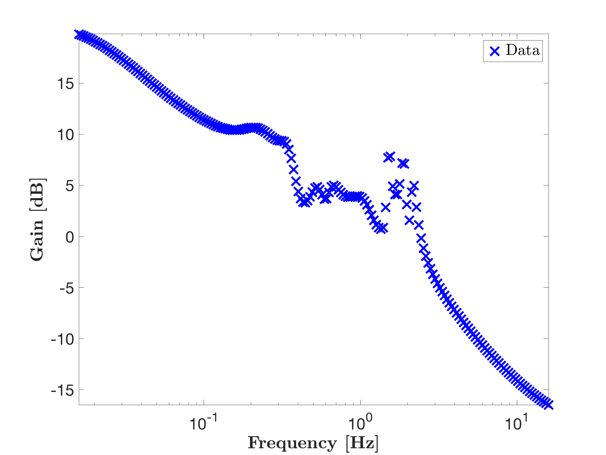
mor.bode({H},'bx',W);

One obtains the following frequency response (called here "data").

Invoking mor.lti, with approximation order objective r = [], as follows:

% Exact interpolation over the complete domain
r             = [];
[sysr1,info1] = mor.lti({W,H},r);

hold on
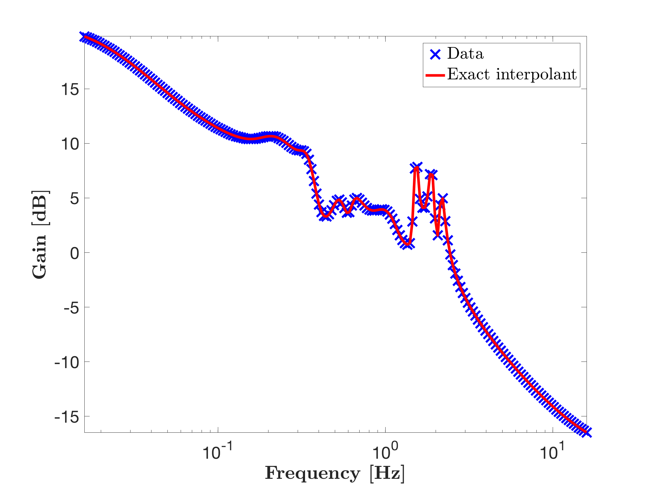
mor.bode(sysr1,'r-',W);
legend('Data','Exact interpolant','Location','NorthEast')

leads to the model sysr1 with realisation of minimial McMillian degree which perfectly interpolates the data. Note that in this case, the order of the realisation is automatically computed. The resulting model sysr1 is given in descriptor form. User can afterward transform it into a non-descriptor form if sysr1.e is full rank.

Now, if an approximate order model of dimenion r = 20 is looked for, the following code should be called,

% Approximate interpolation
r             = 20;
[sysr2,info2] = mor.lti({W,H},r);

hold on
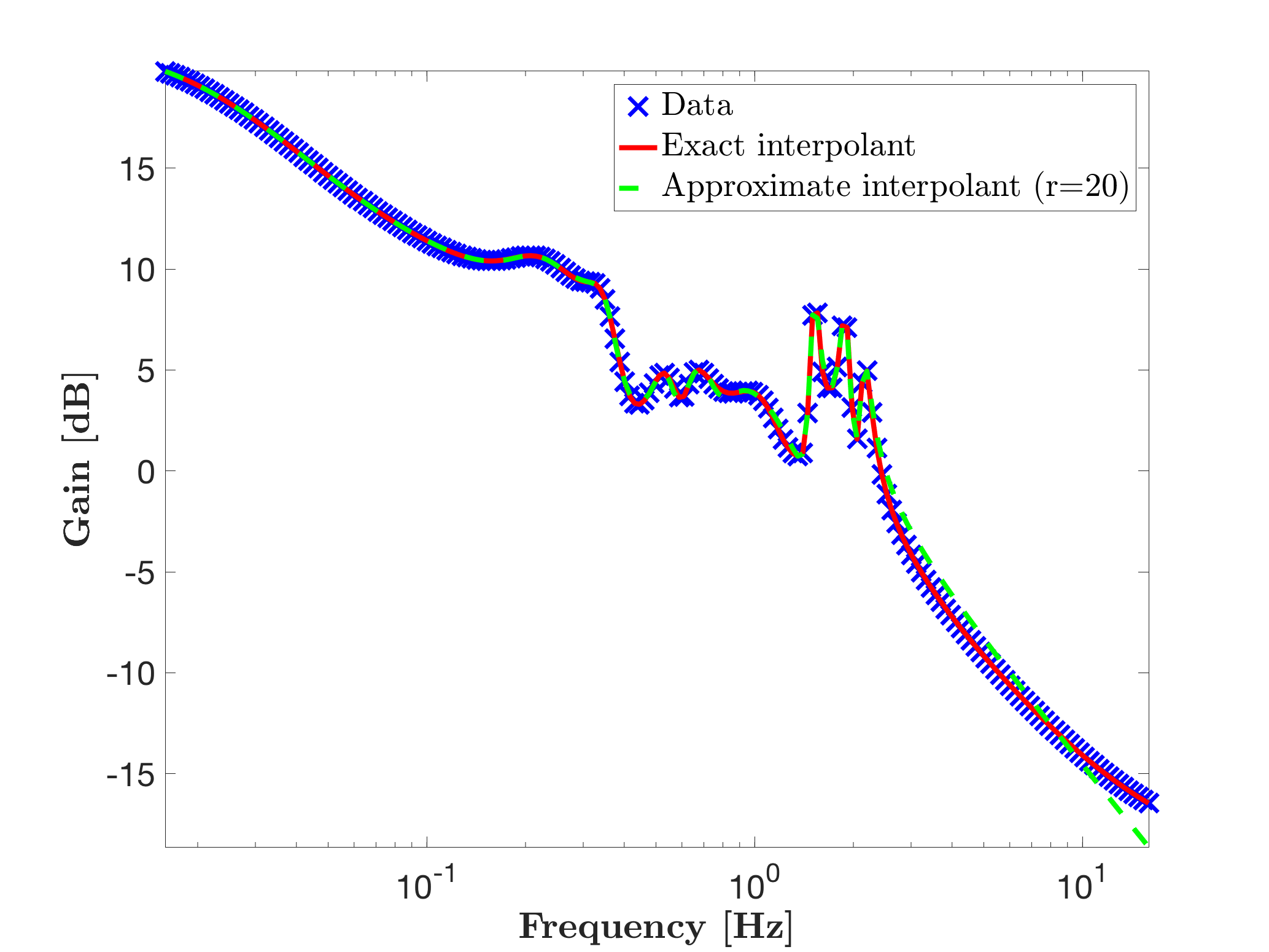
mor.bode(sysr2,'g--',W);
legend('Data','Exact interpolant',['Approximate interpolant (r=' num2str(r) ')'],'Location','NorthEast')

Providing then sysr2, a 20-th order model with a quite good accuracy.