Problem description

Let us be given a set of input-output frequency-domain data, the objective is to find an exact interpolating model over all the frequency range and over a limited one (e.g. from 1 to 10 Hz). Let us define the single input single output random system and evaluate its transfer function response from 0.1 to 100 rad/s as.

% Random stable states-space model and frequency evaluation
rng(1234,'twister');
sys = rss(300,1,1);
sys = stabsep(sys,stabsepOptions('Offset',1e-2));
W   = logspace(-1,2,500);
H   = freqresp(sys,W);

figure
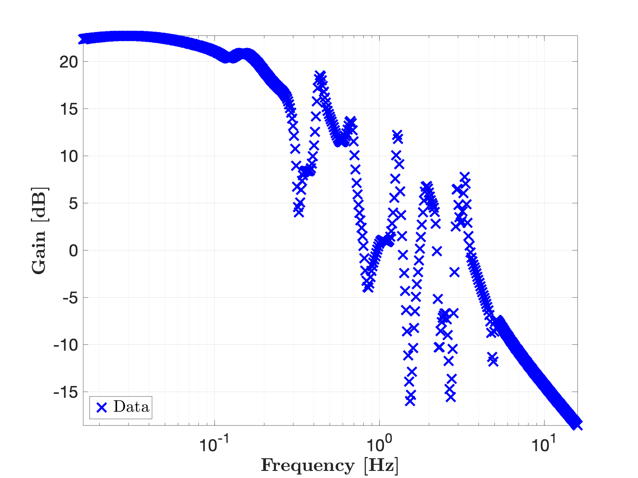
mor.bode({H},'bx',W);
legend('Data','Location','SouthWest')

One obtains the following frequency responses:

Invoking mor.lti, with approximation order objective r = 30, as follows:

% Reduced interpolation over the complete frequency domain
r             = 30;
[sysr1,info1] = mor.lti({W,H},r);

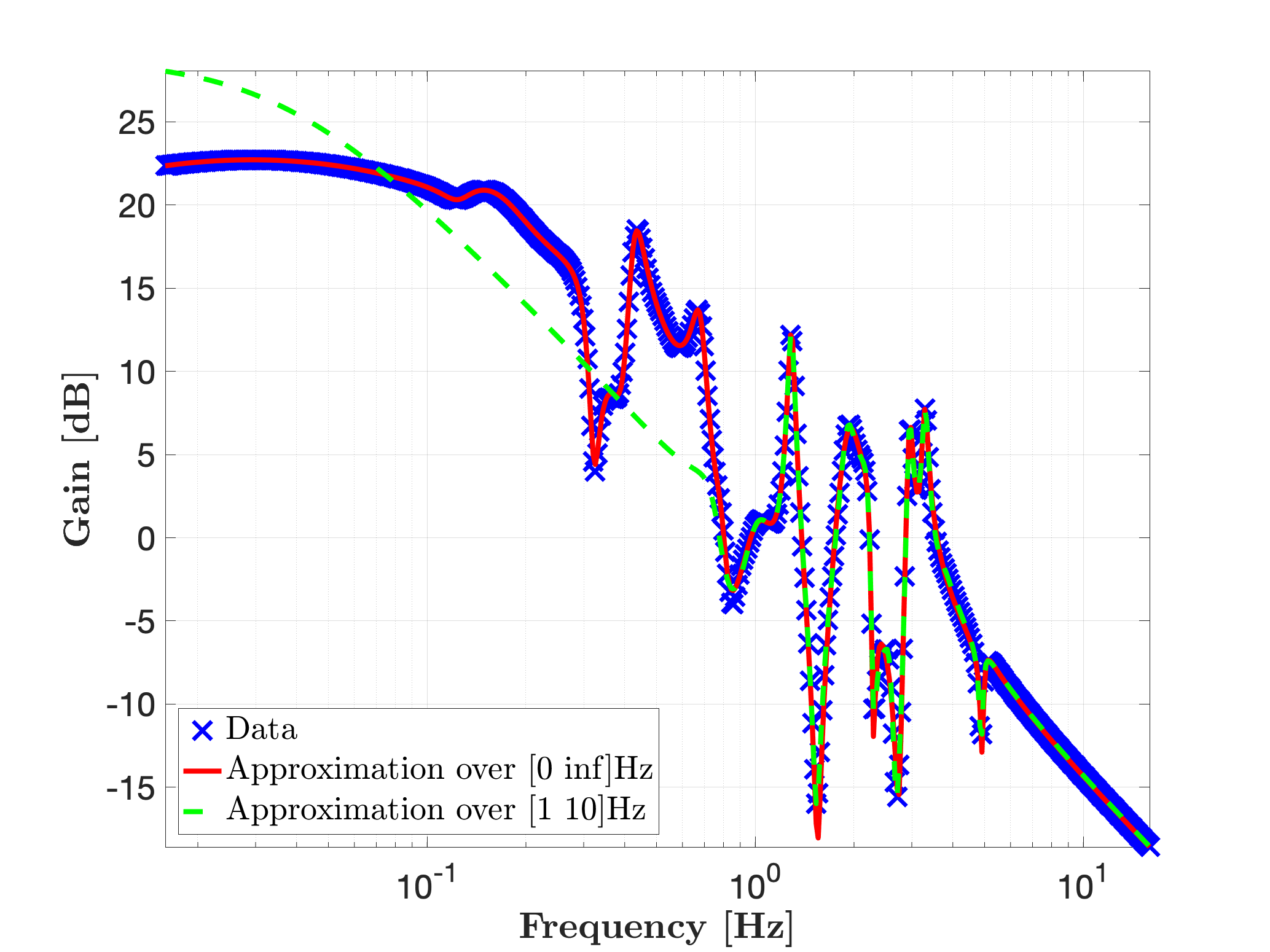
leads to the model sysr1 with realisation of dimension 30. Now, if a limited frequency range (e.g. from 1 to 10 Hz) is of interest only,

% Reduced interpolation over the frequency limited domain [1 10]Hz
opt.freqBand  = [1 10]*2*pi;
[sysr2,info2] = mor.lti({W,H},r,opt);

hold on
mor.bode(sysr1,'r-',W);
mor.bode(sysr2,'g--',W);
legend('Data','Approximation over [0 inf]Hz','Approximation over [1 10]Hz','Location','SouthWest')

leads to the model sysr2 with realisation of minimial McMillian degree which perfectly interpolates the data over this limited frequency range.

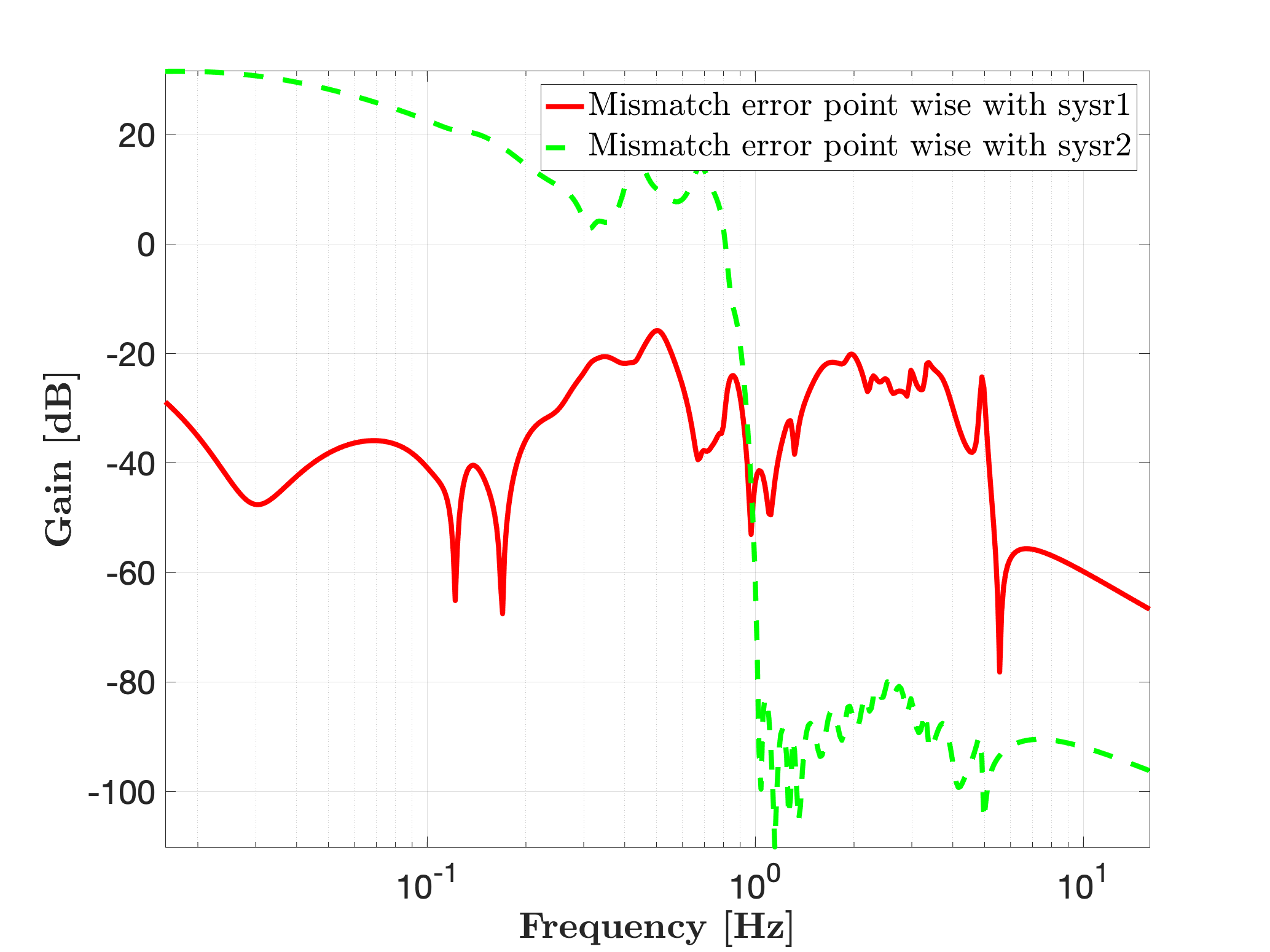
Then, the resulting state-space models are with the following dimensions. The mismatch error can also be analysed.

size(sysr1) % State-space model with 1 outputs, 1 inputs, and r states.
size(sysr2) % State-space model with 1 outputs, 1 inputs, and r states.

figure, hold on
mor.bode(sys-sysr1,'r-',W);
mor.bode(sys-sysr2,'g--',W);
legend('Mismatch error point wise with sysr1','Mismatch error point wise with sysr2','Location','NorthEast')