Problem description

Let us be given a set of input-output frequency-domain data, subject to noise, the objective is to find an exact stable interpolating model. Let us define the single input single output random stable system and evaluate its transfer function response, from which noise is artificially added as.

% Random 100-states model and frequency evaluation
rng(1234,'twister');
sys = rss(100,1,1);
sys = stabsep(sys); % the stable part is kept only
W   = logspace(-1,2,100);
H   = freqresp(sys,W);
% Let consider some noise on the frequency responses
H(1,1,:) = squeeze(H(1,1,1:numel(W))) .* (1 + .05*randn(numel(W),1));

figure
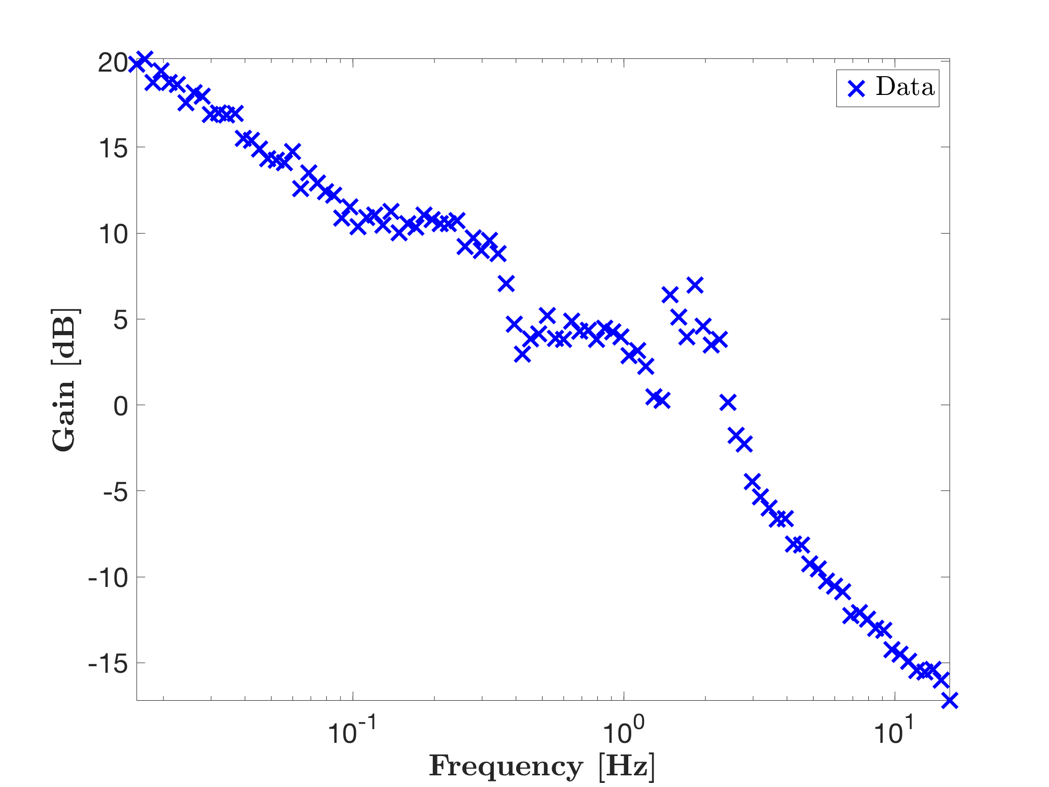
mor.bode({H},'bx',W);
legend('Data','Location','NorthEast')

One obtains the following noisy frequency responses.

Invoking mor.lti, with approximation order objective r = [], as follows

% Exact interpolation
r             = [];
[sysr1,info1] = mor.lti({W,H},r);
isstable(sysr1)

hold on
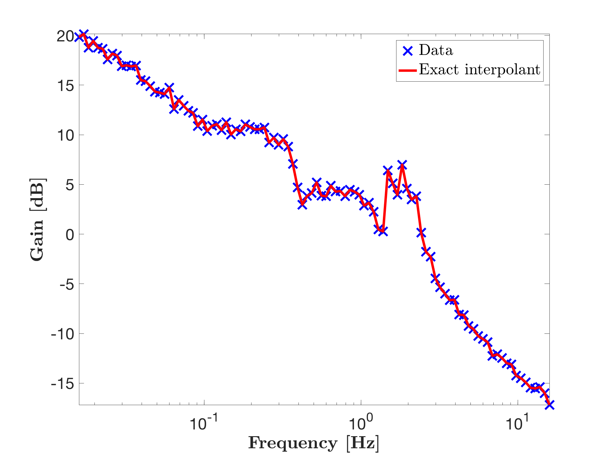
mor.bode(sysr1,'r-',W);
legend('Data','Exact interpolant','Location','NorthEast')

leads to the model sysr1 with realisation of minimial McMillian degree which perfectly interpolates the data. Note that in this case, the order is automatically computed. In addition, in this case, the resultig model might be unstable, even is the original model is stable (this is caused by the interpolatory framework which also catches the noise).

Then, using the optional argument opt.ensurestab = true, with approximation order objective r = [], as follows:

% Exact interpolation with stability enforcement
opt.ensureStab = true;
[sysr2,info2]  = mor.lti({W,H},r,opt);
isstable(sysr2)

hold on
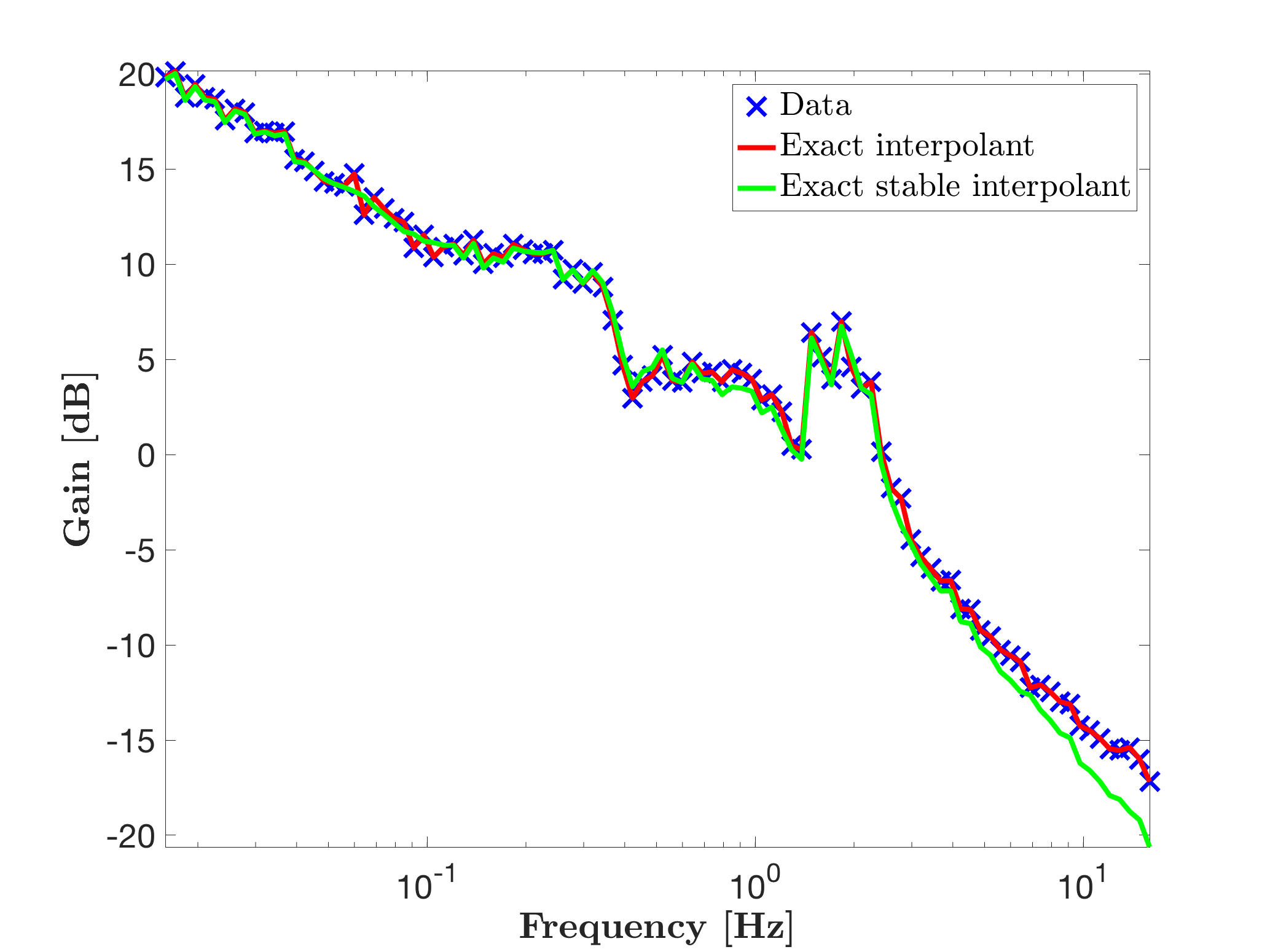
mor.bode(sysr2,'g--',W);
legend('Data','Exact interpolant','Exact stable interpolant','Location','NorthEast')

leads to the model sysr2 with realisation of minimial McMillian degree which interpolates the data and which is stable.