Problem description

Let us be given a (potentially complex) time-domain simulator, which can be simulated on-demand by the user, the objective is to seek for a linear model, reproducing the behaviour of the simulator. Let start by defining a linear model and simulate its response to a frequency chirp.

% Random stable model generation
rng(1208,'multFibonacci');
sys = stabsep(rss(100,2,1));
Tf  = 10;

% Impulse response of this model
figure(1)
mor.impulse(sys,'b-',Tf)
legend('Real model','Location','South')

% Evaluation of the time response using a frequency chirp going from F0 to F1, with a sampling period of Te
Te = 2e-2;
T  = 0:Te:4*Tf;
F0 = 1e-3;
F1 = 2/Te;
T1 = T(end);
U  = chirp(T,F0,T1,F1);
Y  = lsim(sys,U,T);

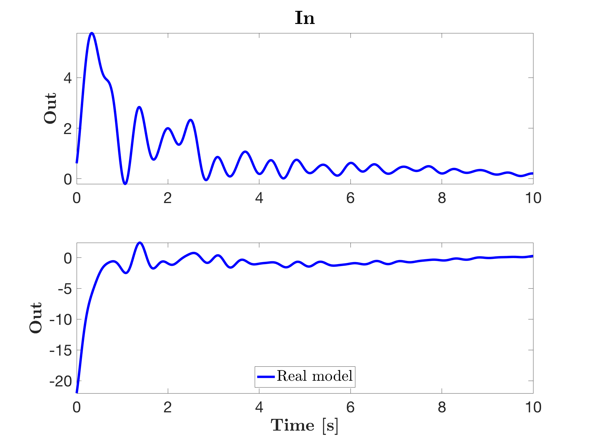
Producing the following impulse response.

Then, after a frequency chirp simulation, it is possible to evaluate the frequency-domain response using a Fourier transform. This can be done using the Signal processing toolbox.

% Evaluate the tranfert function frequency domain response (this is done using the tfestimate function, embedded in the Signal processing toolbox, but other method can be used, e.g. FFT)
[Txy,F]  = tfestimate(U,Y,[],[],[],1/Te);
H(1,1,:) = Txy(:,1);
H(2,1,:) = Txy(:,2);
F        = F(1:end);
W        = 2*pi*F;
size(W)

figure(2)
mor.bode({H},'bx',W)
legend('Data','Location','South')

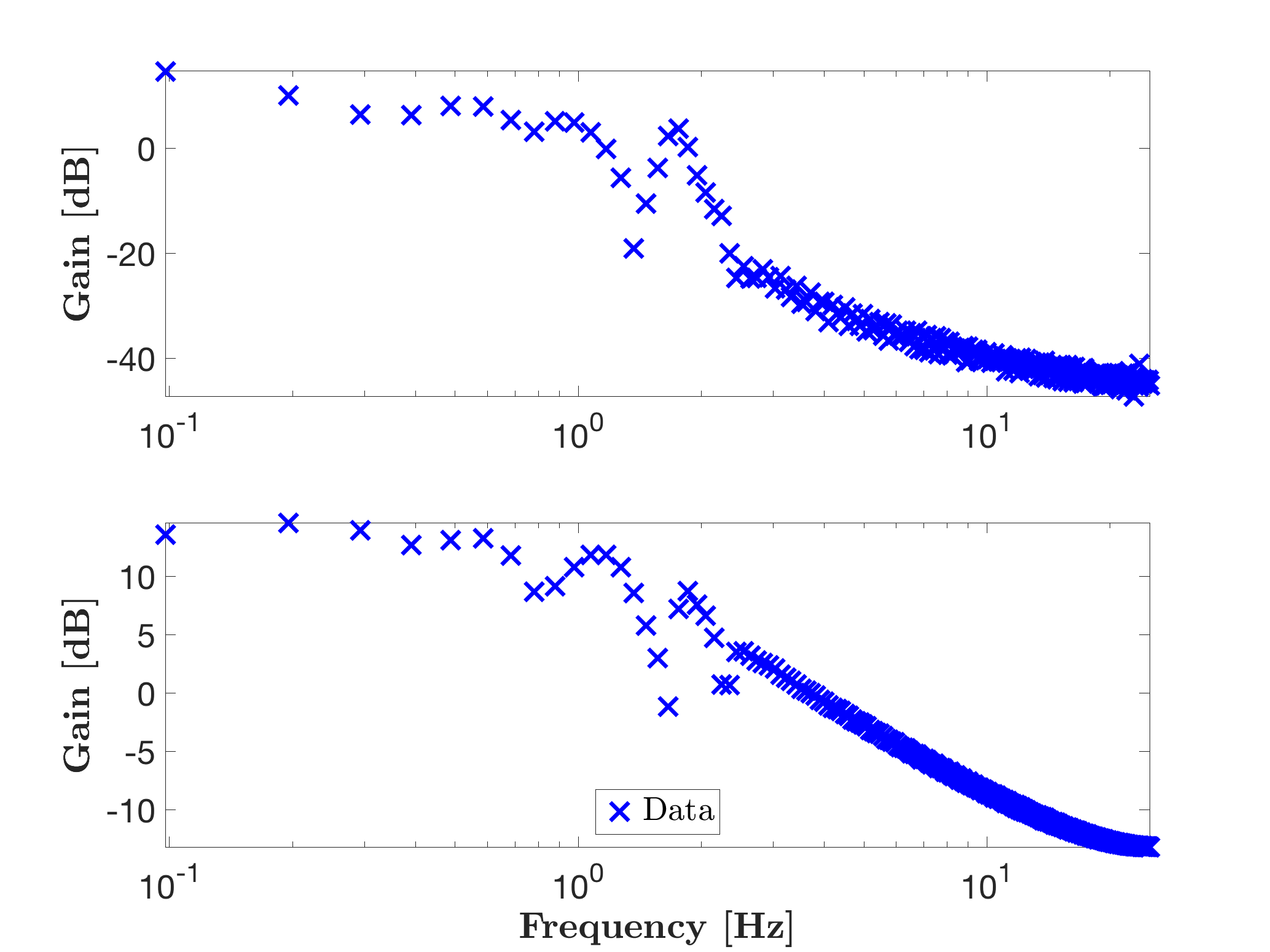
Then one obtains the following figure, illustating the transfer response over the frequency range defined by F.

Invoking mor.lti, with approximation order objective r = [], as follows:

% Exact interpolation can be of large order due to the number of frequency samples (i.e. size(W)).
r             = [];
[sysr1,info1] = mor.lti({W,H},r);
size(sysr1)
isstable(sysr1)

leads to the model sysr1 that exactly interpolates the original data. Note that, since the frequency data are the result of a FFT computation over a frequency signal which is not necessarily persistently exciting, the data are noisy, and the resulting model is here unstable. However, the original system was stable. Now, let us enforce the stability and generate sysr2, and compute its corresponding impulse and Bode responses.

% And now a stable one...
opt.ensureStab = true;
[sysr2,info2]  = mor.lti({W,H},r,opt);
size(sysr2)
isstable(sysr2)

figure(1), hold on
mor.impulse(sysr2,'r-',Tf);
legend('Real model','Exact stable interpolant','Location','South')

figure(2), hold on
mor.bode(sysr2,'r-',W);
legend('Data','Exact stable interpolant','Location','South')

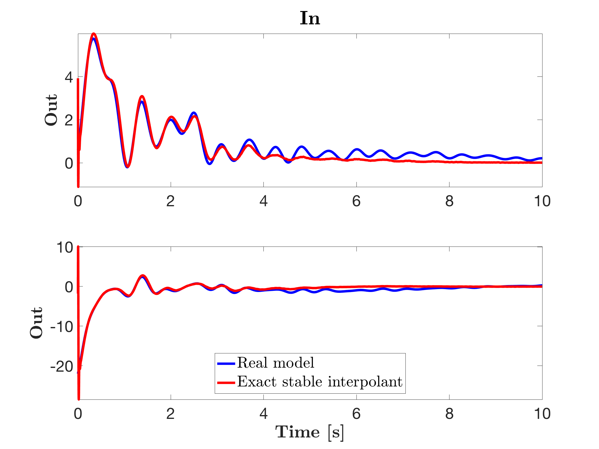
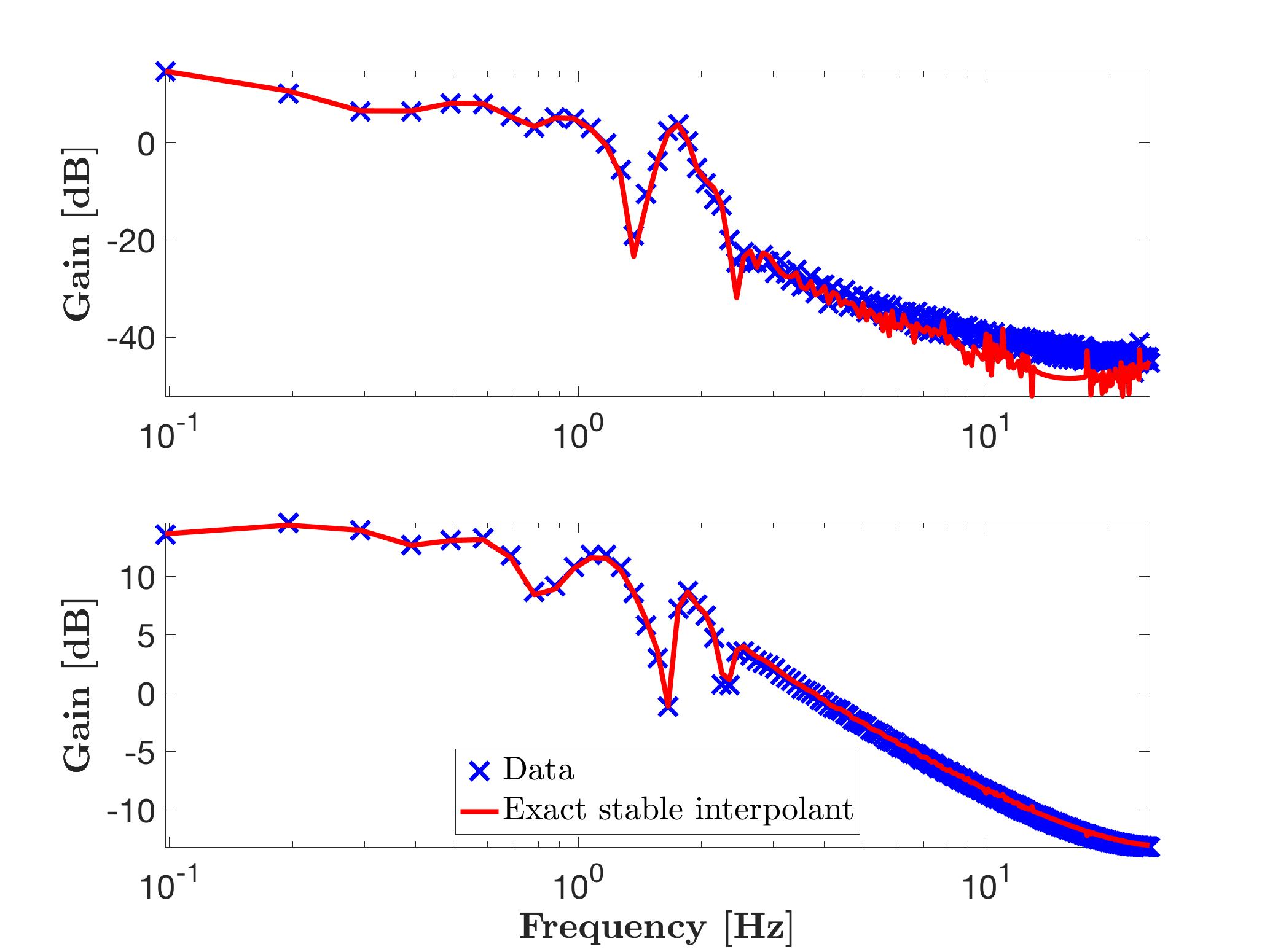
The sysr2 model is stable, but since the interpolating model also catches the high frequency numerical noise, let us approximate it with a reduced order model of dimension r=30, as follows, leading to the following results.

% And now let's try a stable lower one, e.g. r = 30...
r             = 30;
[sysr3,info3] = mor.lti({W,H},r,opt);
size(sysr3)
isstable(sysr3)

figure(1), hold on
mor.impulse(sysr3,'g--',Tf);
legend('Real model','Exact stable interpolant',['Approximate stable interpolant, r = ' num2str(r)],'Location','South')

figure(2), hold on
mor.bode(sysr3,'g--',W);
legend('Data','Exact stable interpolant',['Approximate stable interpolant, r = ' num2str(r)],'Location','South')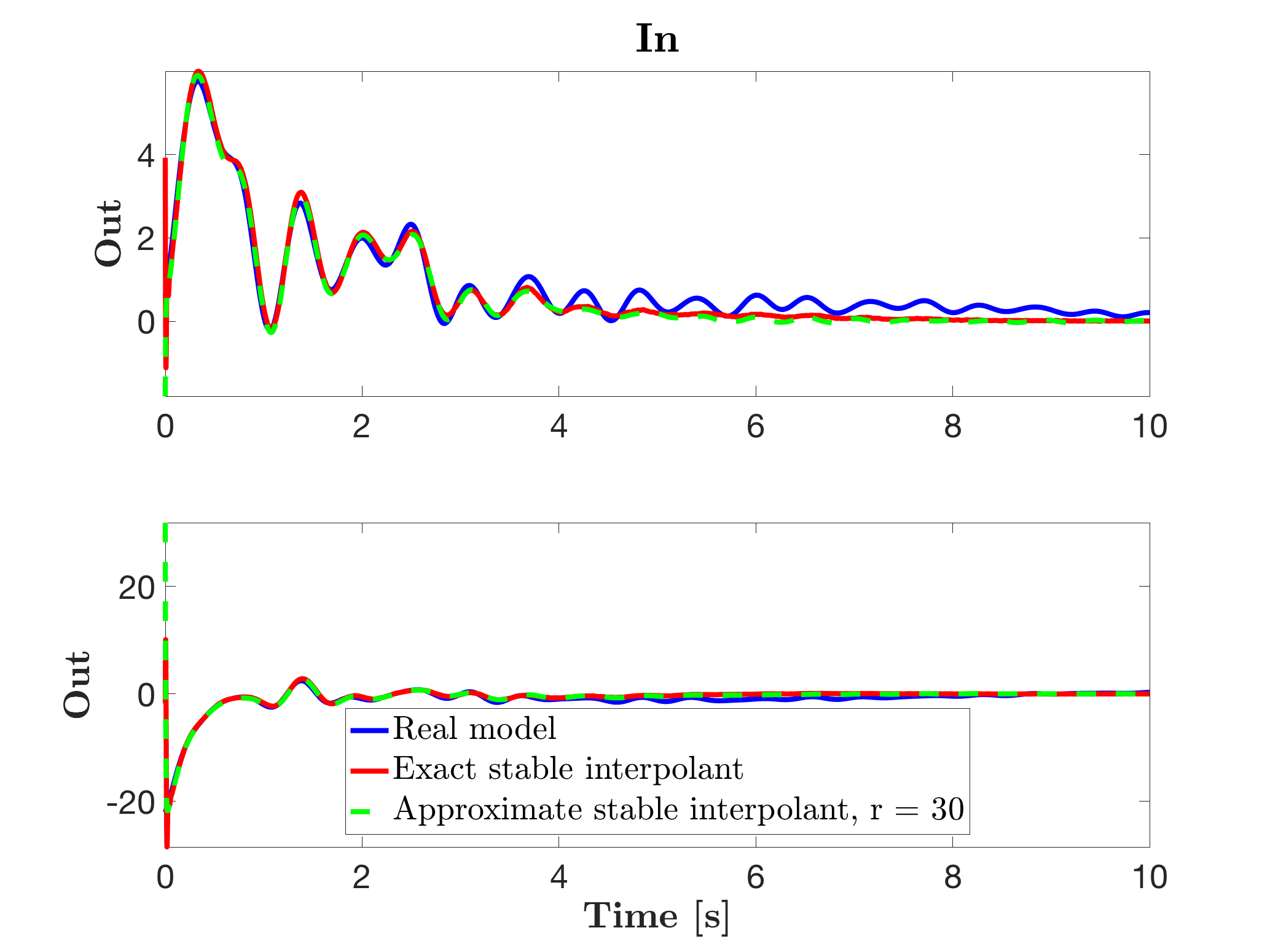

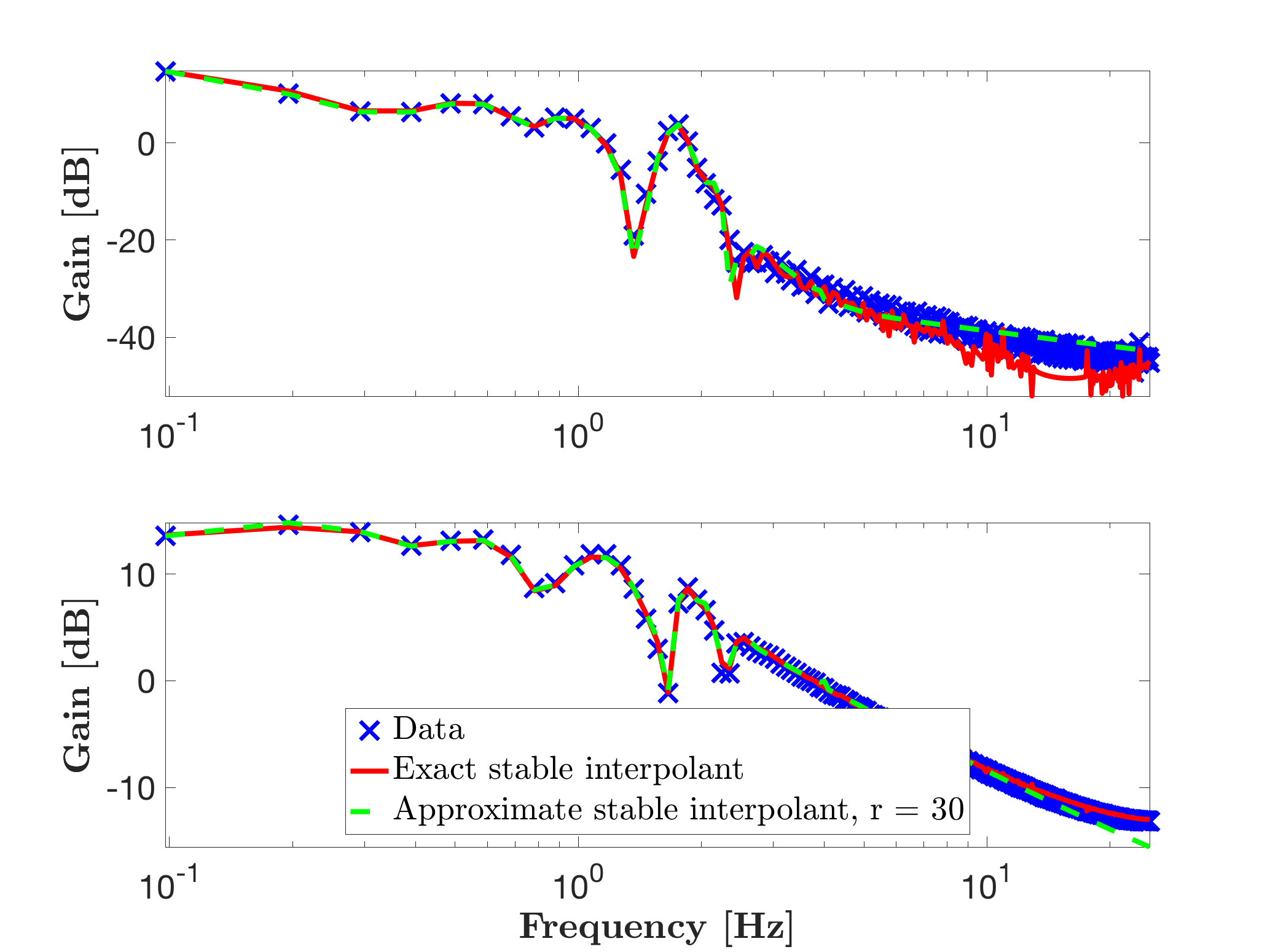
Which leads to sysr3, a stable and simple model that quite well reproduces the original model impulse response, althrough no information where initially available.