mor.bodeDamp

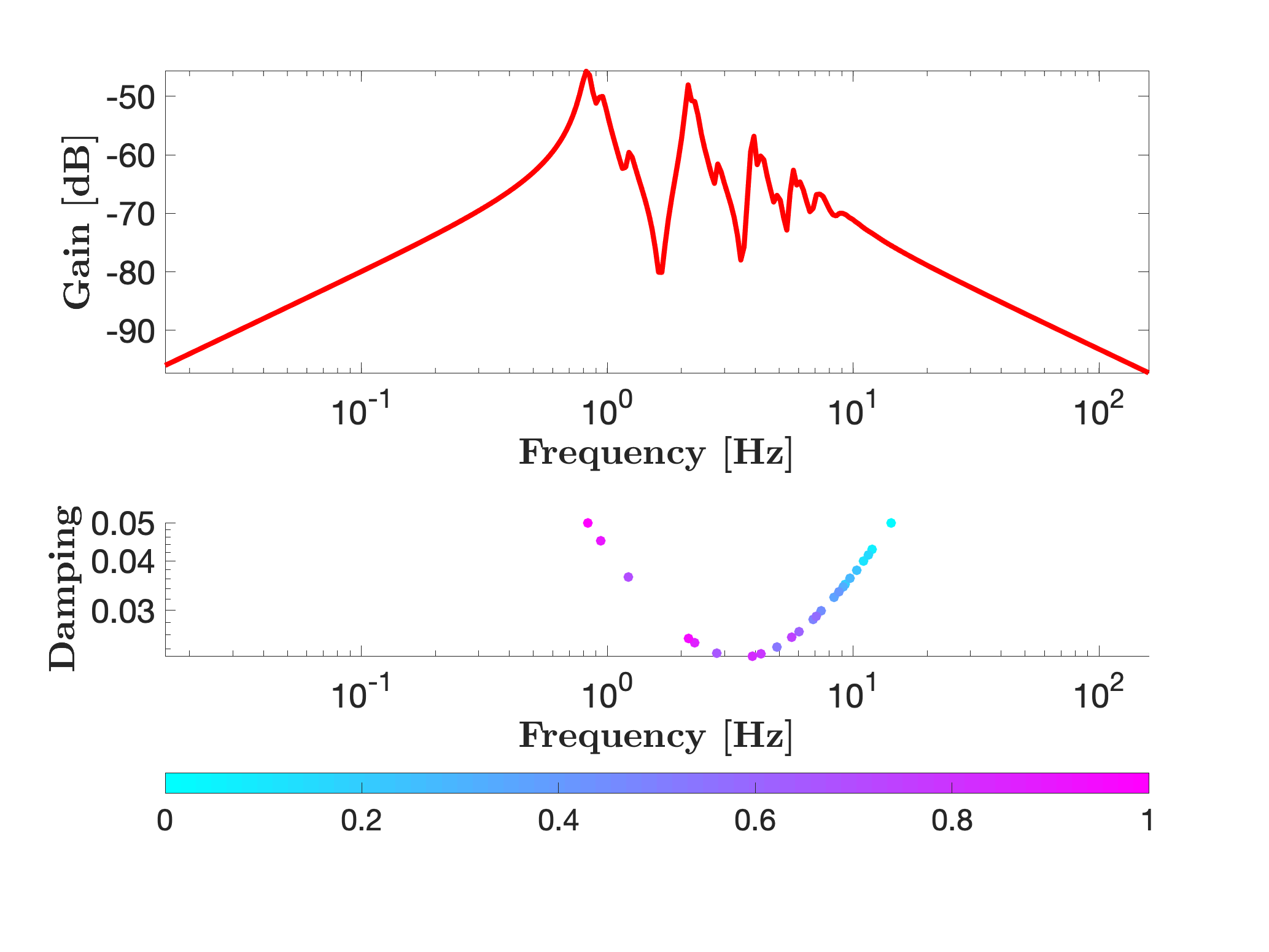
Main interface for SISO Bode and damping map plot of a single model.

Syntax

mor.bodeDamp(sys,W)
mor.bodeDamp(sys,color,W)

Description

mor.bodeDamp(sys,W) plots the SISO Bode diagram and the associated damping map of sys over the frequencies defined by the vector W. The plot shows the frequency response and related eigenvalues frequencies and damping, as a function of their associated residue. Black crosses gives the unstable modes. The input sys can either be

a state-space ODE (DAE) realization described as sys = ss(A,B,C,D) (or sys = dss(A,B,C,D,E))
a matrix set describing an ODE (or DAE) described as sys = {A,B,C,D} (or sys = {A,B,C,D,E})

mor.bodeDamp(sys,color,W) plots sys with color color.

Input arguments

sys	Dynamical system or input-output data. More specifically `sys` can either be a state-space ODE (DAE) realization described as `sys = ss(A,B,C,D)` (or `sys = dss(A,B,C,D,E)`) a matrix set describing an ODE (or DAE) described as `sys = {A,B,C,D}` (or `sys = {A,B,C,D,E}`)
color	Color in a string tag or a RGB vector.
W	Vector of frequencies, in rad/s, over which the system's frequency responses are evaluated (positive real vector).

Output arguments

none

Examples

% Bode and damping from state-space
load build
W = logspace(-1,3,300);
figure
mor.bodeDamp(G,W)

The above script generates the following figure, where the up frame represents the frequency response of the SISO model and the down frame illustrates the eigenevalues equivalent frequency and damping values. The color are function of residue value associated with the eigenvalue. It reveals somehow the importance of the eigenvalue.