Problem description
Let us be given a state-space model described by an ODE set, the objective is to find an approximate reduced order model, using different options and features of the MOR Toolbox. Let us get the state-space model included in MATLAB, representing a building model.
% Obtain a state-space test model
load build
sys = G;
W   = logspace(-1,3,300);
size(sys) % SISO model with state-space dimension = 48

figure
mor.bode(sys,'b-',W);
legend('Original model','Location','South')
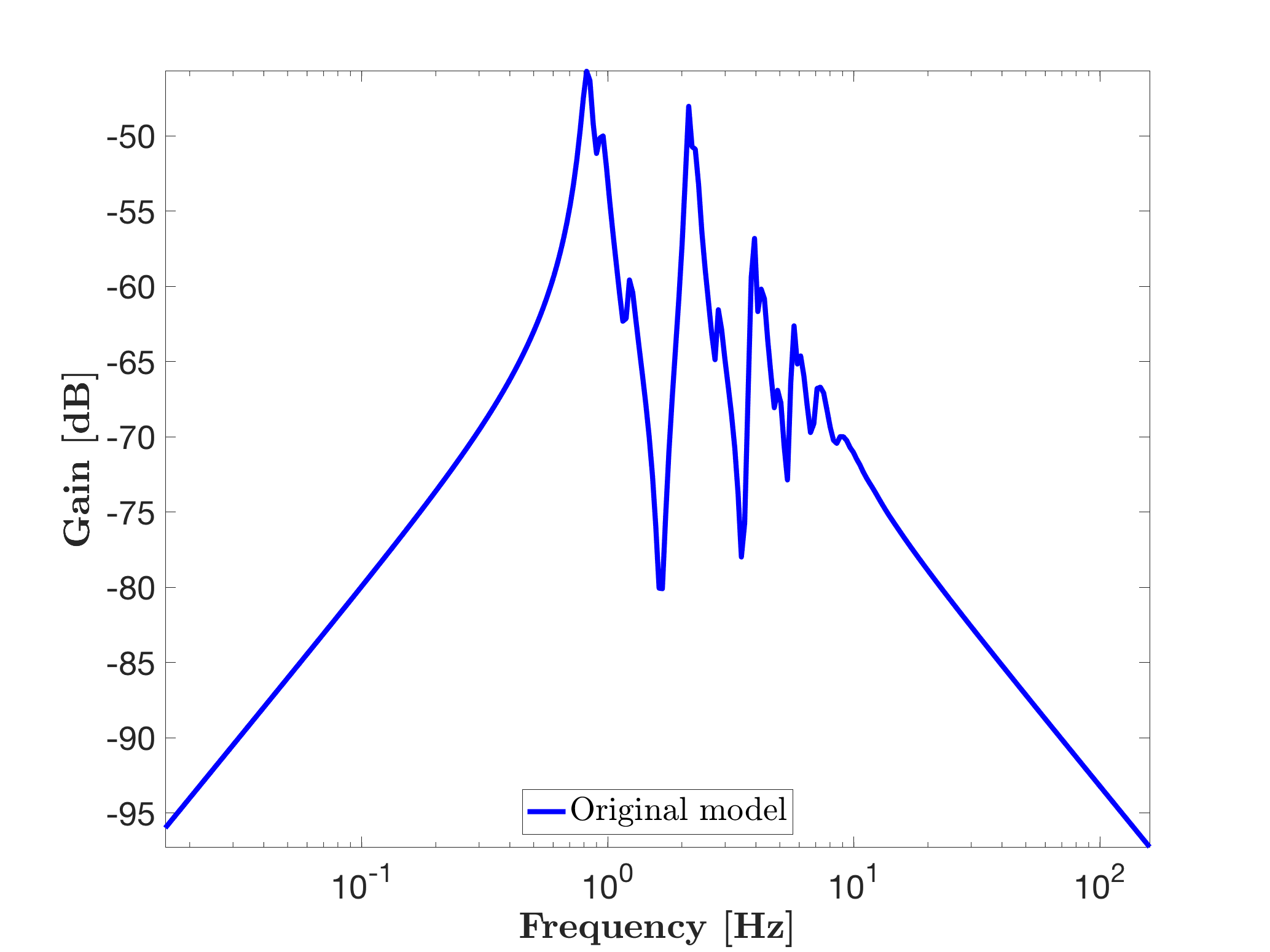
One obtains the following frequency response (called here "Original model").

Invoking mor.lti, with approximation order objective r = 10, as follows:
% Reduction with no options (and default tuning)
r     = 10;
sysr1 = mor.lti(sys,r);

hold on
mor.bode(sysr1,'g--',W);
legend('Original model',['Approximate model (r=' num2str(r) ')'],'Location','South')
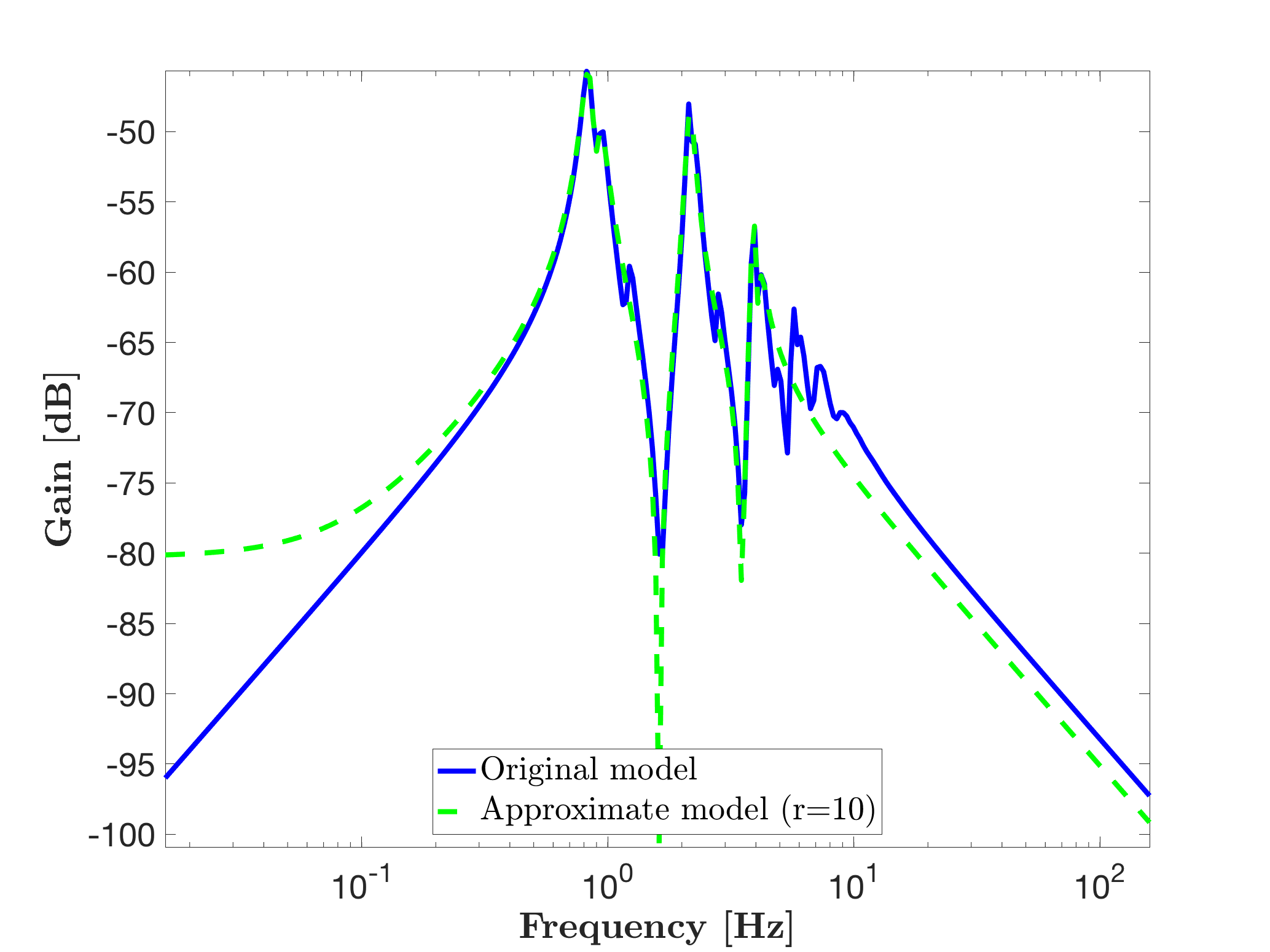
leads to the model sysr1 with state-vector of dimension 10. It results in the following Bode response.

Here, the default options are used. If one is now interested in obtaining the approximation process informations and modify the stopping convergence criteria, the following fields can be set.
% Reduction with visualisation and information options plus a different tolerance level
opt.verbose   = true; % shows the iterations
opt.extraInfo = true; % provides additional informations
opt.tol       = 1e-3; % relative change in interpolation points tolerance
[sysr2,info2] = mor.lti(sys,r,opt);
info2.sigma % are the optimal interpolation points
info2       % are the output informations
Leading to the following informations, describing the invoked method (here ISTIA), the original and reduced order models, the mismatch H2 norm error checking, the frequency range of interest and the shift selection approach. Then, the iterations are displayed. Here, the process converges in 13 iterations.
+------------------------------------------------------------------------------+
| MOR Toolbox Dev version                                                      |
| ISTIA - Iterative SVD-Tangential Interpolation Algorithm                     |
+------------------------------------------------------------------------------+
| Original system      : 48 states, 1 input(s), 1 output(s)                    |
| Reduced system order : 10                                                    |
| H2(W) norm error     : not checked                                           |
| Frequency bound      : [0 Inf] rad/s                                         |
| Shift selection      : automatic                                             |
| Start: 1 /1                                                                  |
|         Iteration             Unconv. shifts               Delta Hr          |
|              1                      10                         -             |
|              2                      10                       0.86            |
|              3                      10                       0.29            |
|              4                       8                       0.24            |
|              5                       6                       0.19            |
|              6                       6                       0.07            |
|              7                       8                       0.11            |
|              8                      10                       0.16            |
|              9                      10                       0.14            |
|             10                      10                       0.11            |
|             11                       6                       0.02            |
|             12                       2                       0.01            |
|             13                       0                       0.00            |
+------------------------------------------------------------------------------+


ans =

1.4278 +34.7678i
0.9064 +24.4610i
0.3723 +14.0577i
0.3361 +13.5280i
0.4304 + 5.2689i
1.4278 -34.7678i
0.9064 -24.4610i
0.3723 -14.0577i
0.3361 -13.5280i
0.4304 - 5.2689i


info2 =

struct with fields:

  success: 1
     iter: 13
stability: 1
        V: [48×10 double]
        W: [48×10 double]
    sigma: [10×1 double]
        L: [1×10 double]
        R: [1×10 double]
The optimal interpolation points are concentrated in the info2.shift. User can view them as points in the complex plane that are important to interpolate in order to match the transfer. Additinal informations, such as the left and right projectors (info2.W and info2.V) and tangential directions (info2.L and info2.R) are provided in info2 (these latter are adapted to expert users).
Now, if one seek for the best model (in the H2-norm mismatch sense), the option opt.checkH2 can be set to true (useful only if original model is stable).
% Reduction with the H2 error whatch option
opt.checkH2   = true; % slows the process (a '*' appear at each improvement)
[sysr3,info3] = mor.lti(sys,r,opt);

hold on
mor.bode(sysr3,'r--',W);
legend('Original model',['Approximate model (r=' num2str(r) ')'],['Approximate model with H2-norm check (r=' num2str(r) ')'],'Location','South')

% Compute the mismatch error
mor.norm(sys-sysr2,2)
mor.norm(sys-sysr3,2)
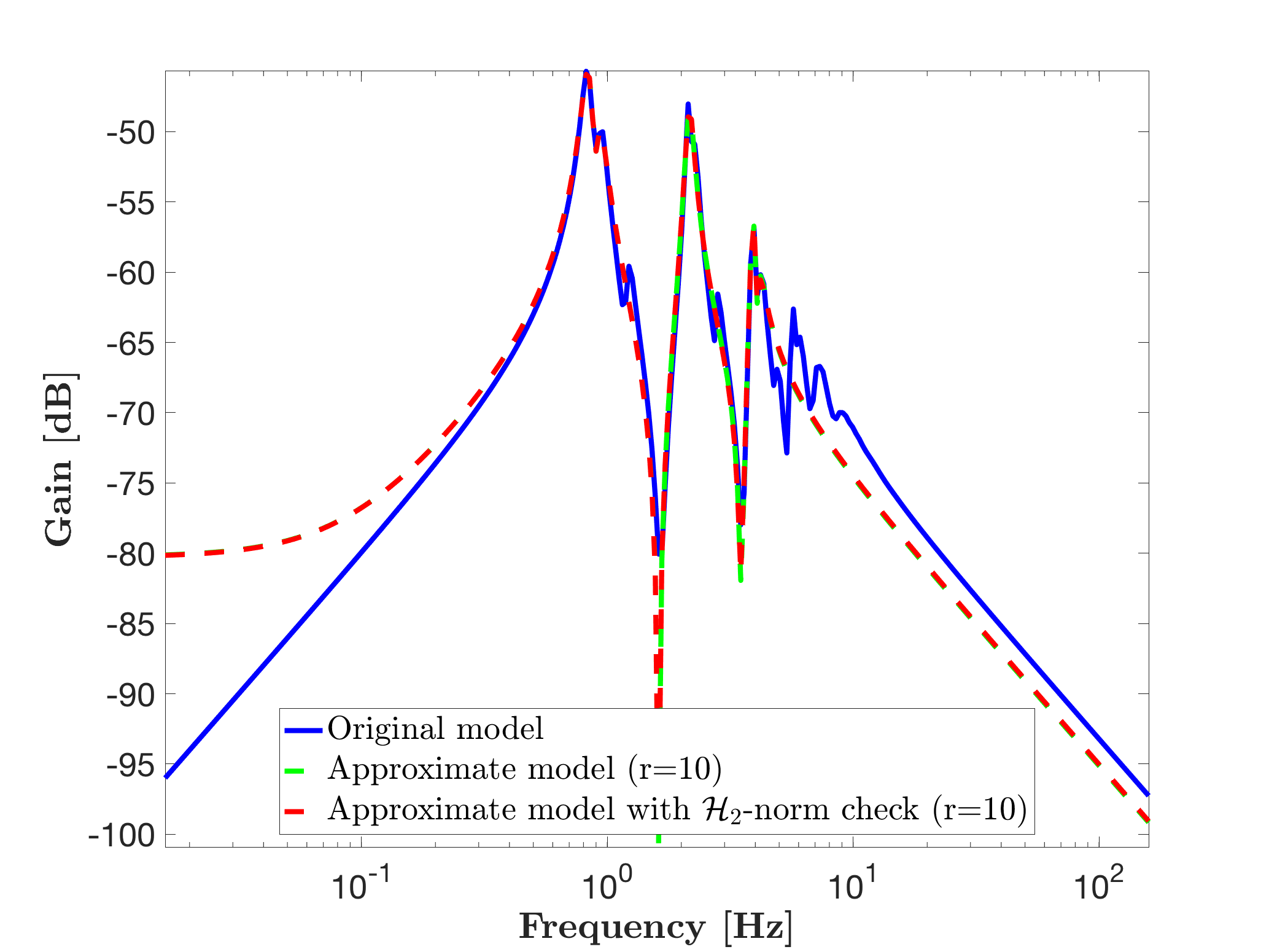
Leading to the following display information and Bode response. In this simple case, the best approximated model is very close to the previous one and is achieved at iteration 11 marked with '*'.
+------------------------------------------------------------------------------+
| MOR Toolbox Dev version                                                      |
| ISTIA - Iterative SVD-Tangential Interpolation Algorithm                     |
+------------------------------------------------------------------------------+
| Original system      : 48 states, 1 input(s), 1 output(s)                    |
| Reduced system order : 10                                                    |
| H2(W) norm error     : checked                                               |
| Frequency bound      : [0 Inf] rad/s                                         |
| Shift selection      : automatic                                             |
| Start: 1 /1                                                                  |
|         Iteration             Unconv. shifts               Delta Hr          |
|              1                      10                         -             |
|            * 2                      10                       0.86            |
|            * 3                      10                       0.29            |
|            * 4                       8                       0.24            |
|            * 5                       6                       0.19            |
|            * 6                       6                       0.07            |
|              7                       8                       0.11            |
|              8                      10                       0.16            |
|              9                      10                       0.14            |
|           * 10                      10                       0.11            |
|           * 11                       6                       0.02            |
|             12                       2                       0.01            |
|             13                       0                       0.00            |
+------------------------------------------------------------------------------+
One can then compare the H2 mismatch error between the two reduced models sysr2 and sysr3 with the original one sys using the mor.norm routine, extending the MATLAB norm function as follows.
% Compute the H2 mismatch error
mor.norm(sys-sysr2,2)
mor.norm(sys-sysr3,2)

ans =

   9.3699e-04


ans =

   9.3356e-04