Problem description

Let us be given a state-space model described by an ODE set, the objective is to find an approximate reduced order model, accurate over a given frequency range, using different options and features of the MOR Toolbox. Let us get the state-space model from the COMPleib library, standardly used in control problems. Once the package obtained, the 'CDP' example can be tested.

% Obtain a state-space test model
[A,B1,B,C1,C,D11,D12,D21,nx,nw,nu,nz,ny] = COMPleib('CDP');
sys  = ss(A,B,C,0);
sys  = sys(1,2);
W    = logspace(-1,6,500);

figure
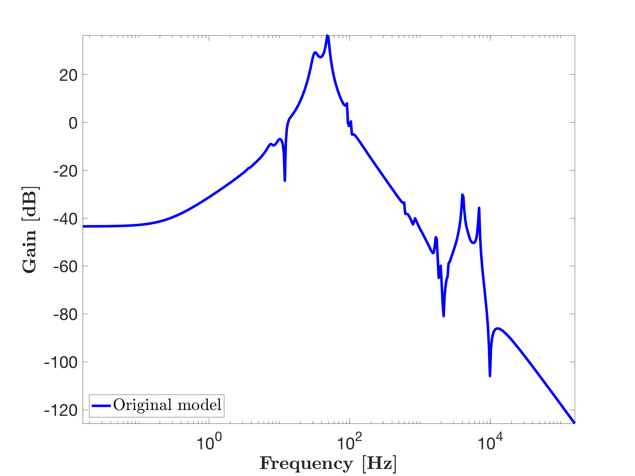
mor.bode(sys,'b-',W);
legend('Original model','Location','SouthWest')

One obtains the following frequency response (called here "Original model").

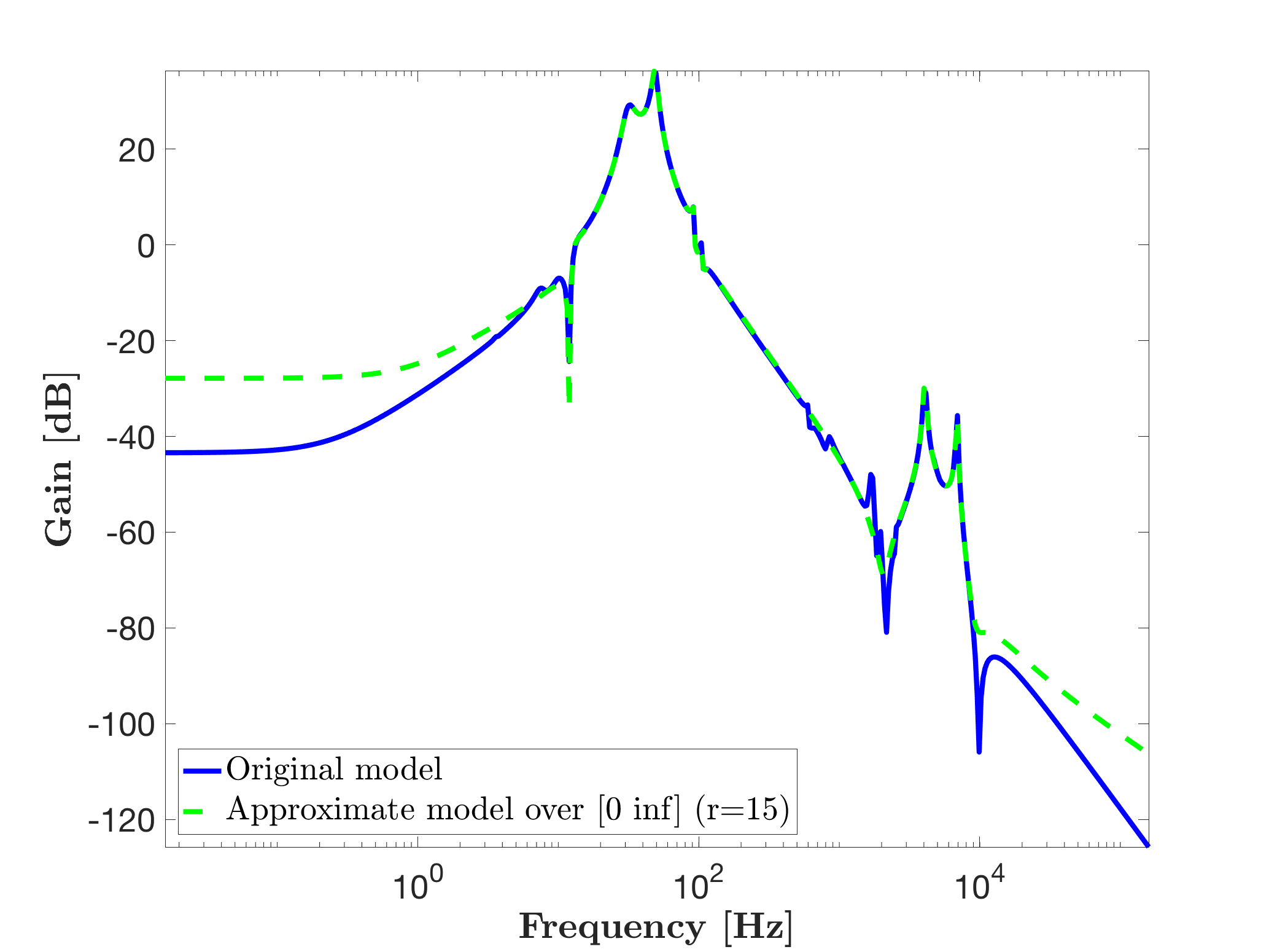
Invoking mor.lti, with approximation order objective r = 15, over the entire frequency range as follows:

% Reduction over [0 inf]rad/s
r           = 15;
opt.verbose = true; % display algorithm iterations
opt.checkH2 = true; % check the H2-norm error at each iterations
sysr1       = mor.lti(sys,r,opt);

hold on
mor.bode(sysr1,'g--',W);
legend('Original model',['Approximate model over [0 inf] (r=' num2str(r) ')'],'Location','SouthWest')

leads to the model sysr1 with state-vector of dimension 15. This leads then to the following Bode response.

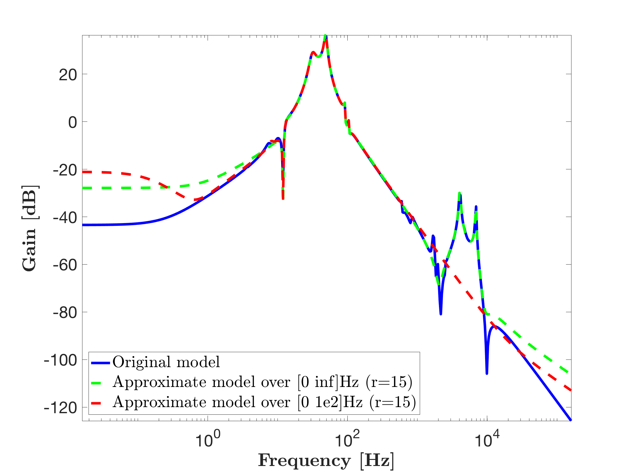
If one is now interested in obtaining the approximation over a finite frequency range, e.g. [0 1e2]*2*pi Hz, the opt.freqBand option can be used as:

% Reduction over a limited frequency range, in rad/s
opt.freqBand  = [0 1e2]*2*pi; % frequency range
[sysr2,info2] = mor.lti(sys,r,opt);

hold on
mor.bode(sysr2,'r--',W);
legend('Original model',['Approximate model over [0 inf]Hz (r=' num2str(r) ')'],['Approximate model over [0 1e2]Hz (r=' num2str(r) ')'],'Location','SouthWest')

Leading to the following Bode response, which clearly now focus on the low frequency, without paying attention to higer frequency peaks.

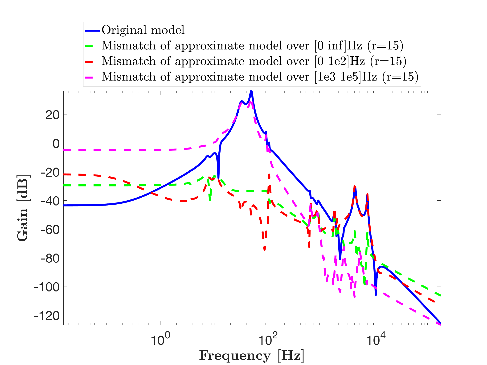
Similarly, one may reduce over the higher frequencies only, e.g. over [1e3 1e5]*2*pi Hz. Then one displays the original system and the approximated mismatch errors for different frequency ranges.

% Reduction over a limited frequency range, in rad/s
opt.freqBand  = [1e3 1e5]*2*pi; % frequency range
[sysr3,info3] = mor.lti(sys,r,opt);

figure
mor.bode(sys,'b-',sys-sysr1,'g--',sys-sysr2,'r--',sys-sysr3,'m--',W);
legend('Original model',['Mismatch of approximate model over [0 inf]Hz (r=' num2str(r) ')'],['Mismatch of approximate model over [0 1e2]Hz (r=' num2str(r) ')'],['Mismatch of approximate model over [1e3 1e5]Hz (r=' num2str(r) ')'],'Location','NorthOutside')

This example illustrates how one can capture a limited frequency behaviour. This feature may be useful when one is interested in simulating or controlling a system within a given frequency working range.