Problem description

Let us be given a state-space model described by an ODE set, the objective is to find an approximate reduced order model, using different options and features of the MOR Toolbox. Let us get the state-space model included in MATLAB, representing a building model.

% Obtain a state-space test model
load build
sys = G;
W   = logspace(-1,3,500);

figure(1)
mor.bode(sys,'b-',W);
legend('Original model','Location','South')

figure(2)
mor.eigen(sys,'b+')
legend('Original model','Location','West')

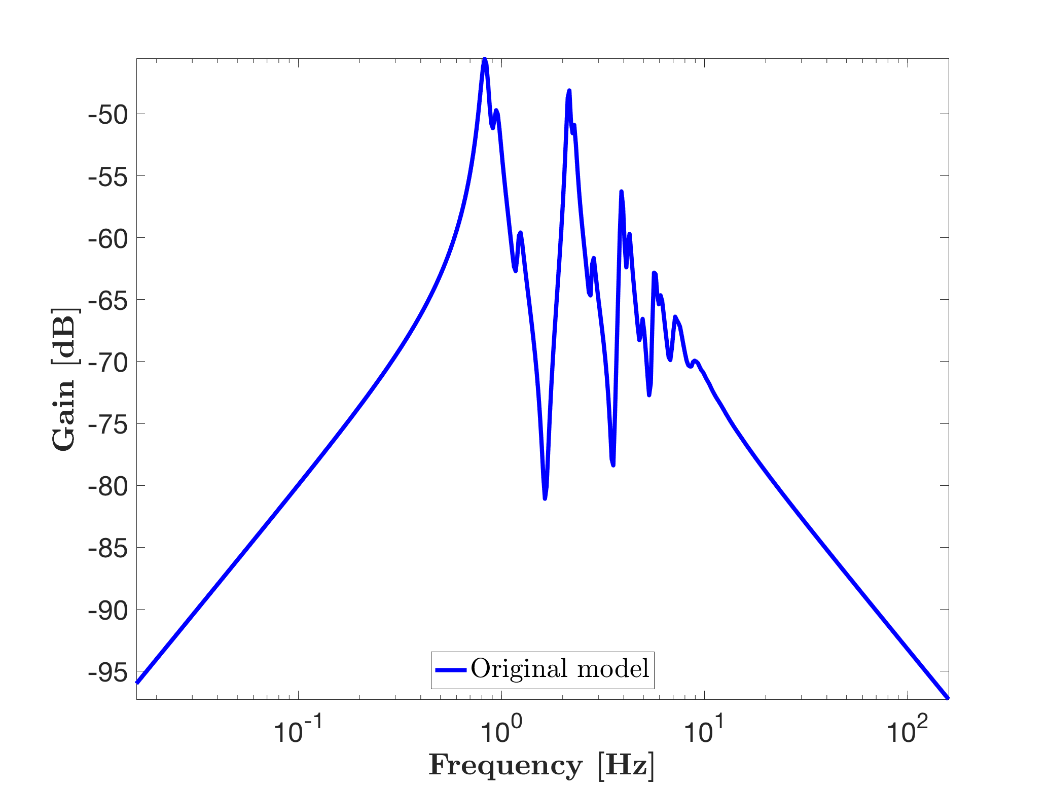
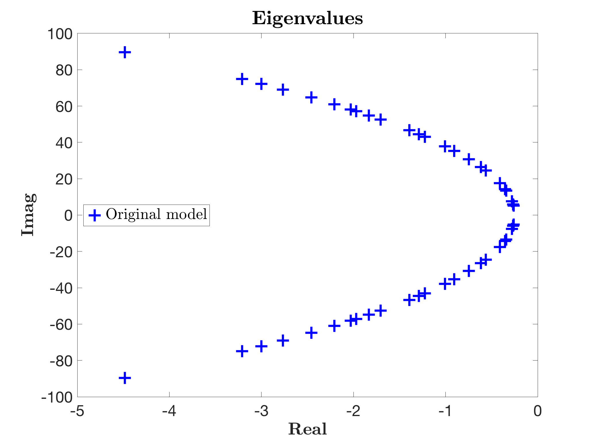
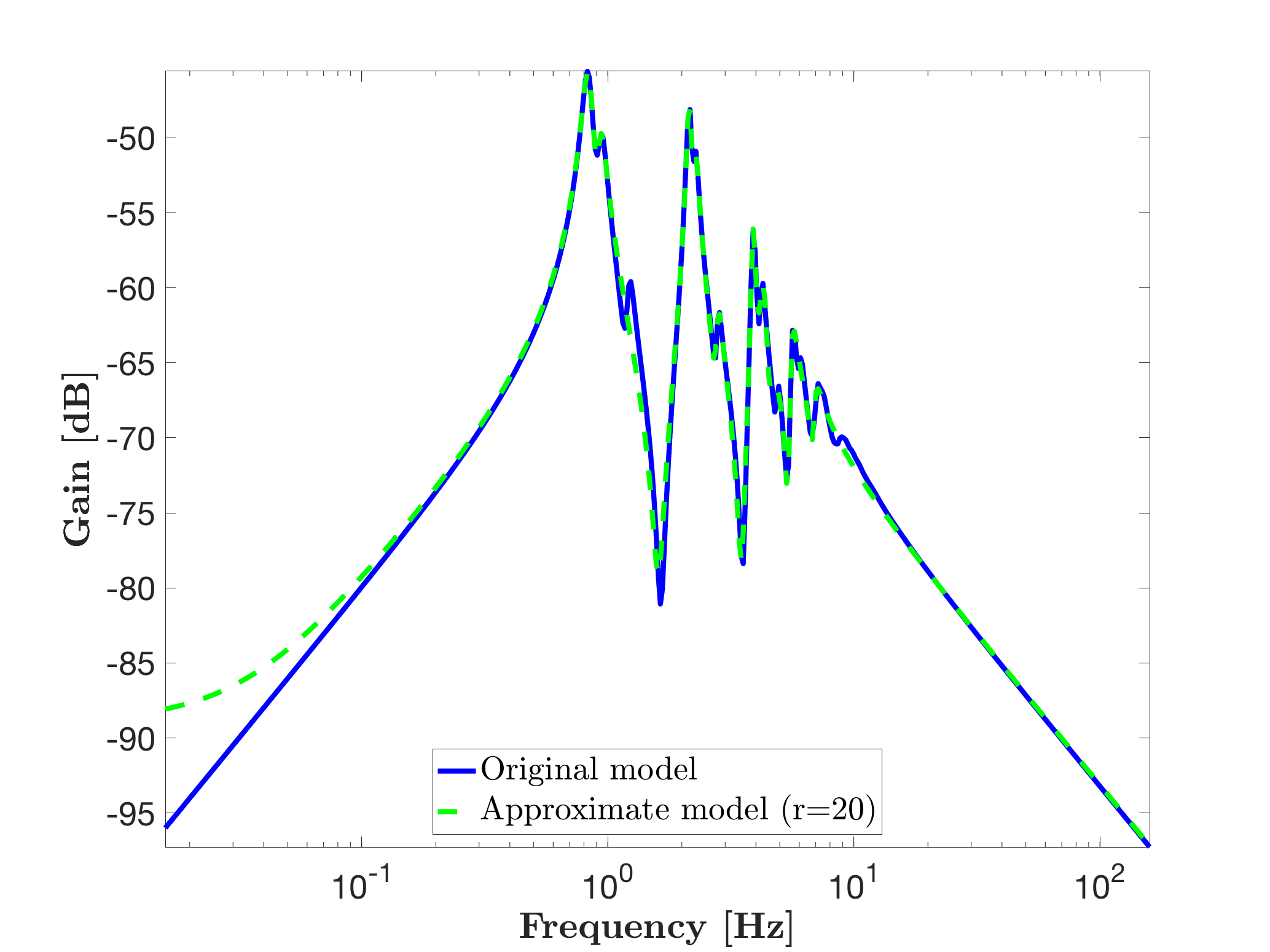
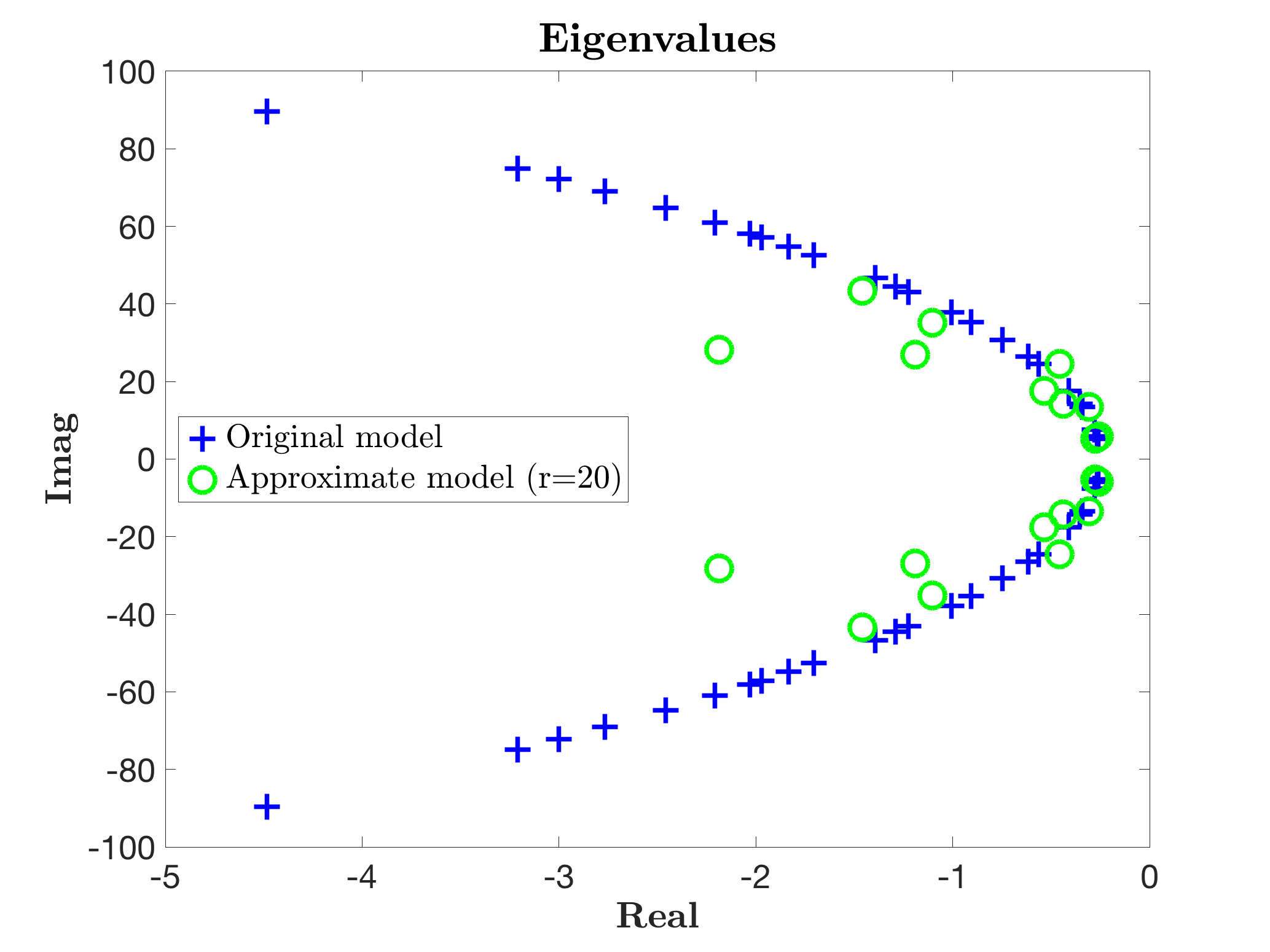
One obtains the following frequency response and eigenvalues (called here "Original model").

Invoking mor.lti, with approximation order objective r = 20, over the entire frequency range as follows:

% Reduction
r              = 20;
opt.verbose    = true;
opt.checkH2    = true;
opt.ensureStab = true;
sysr1          = mor.lti(sys,r,opt);

figure(1), hold on
mor.bode(sysr1,'g--',W);
legend('Original model',['Approximate model (r=' num2str(r) ')'],'Location','South')

figure(2), hold on
mor.eigen(sysr1,'go')
legend('Original model',['Approximate model (r=' num2str(r) ')'],'Location','West')

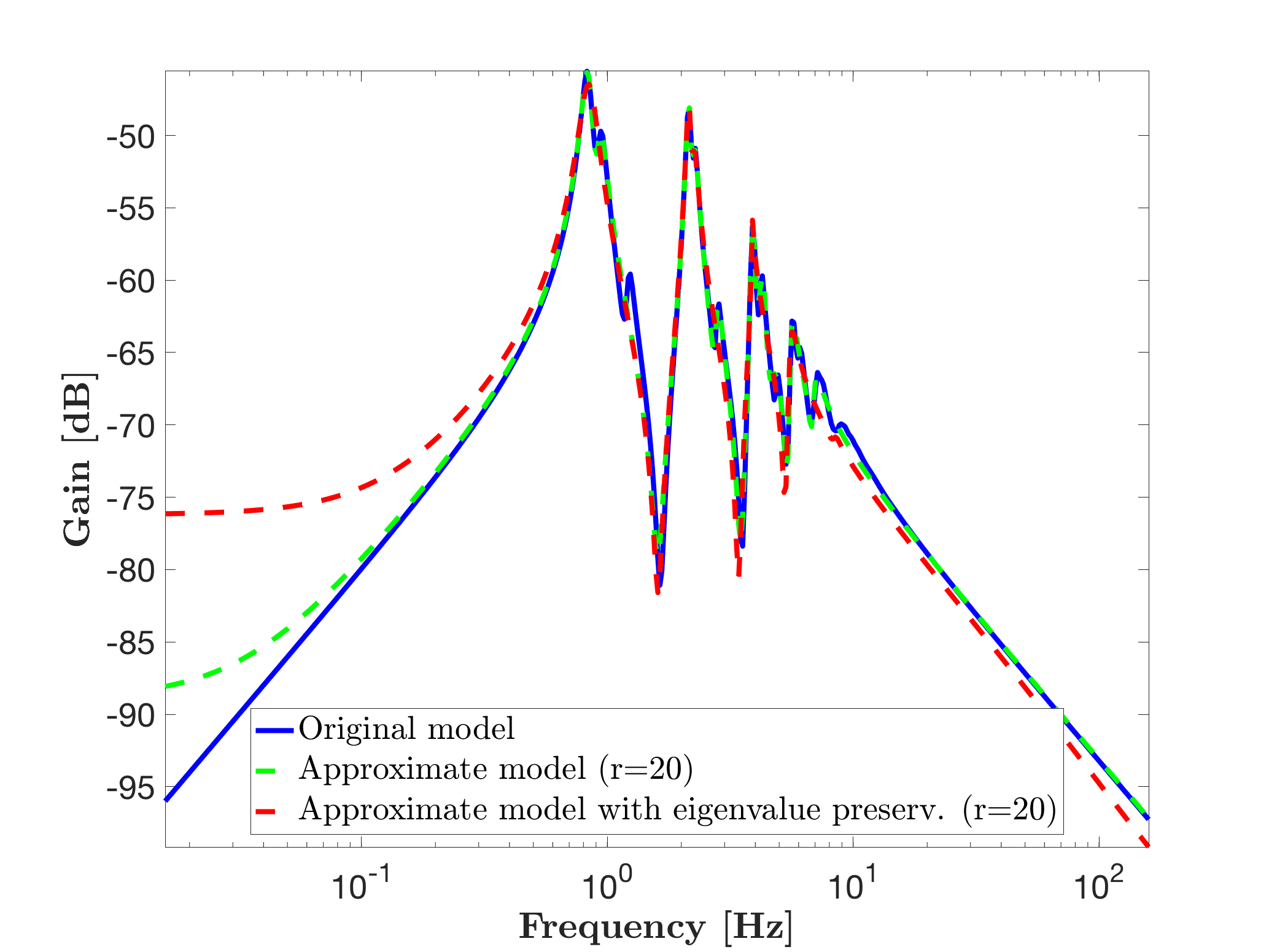
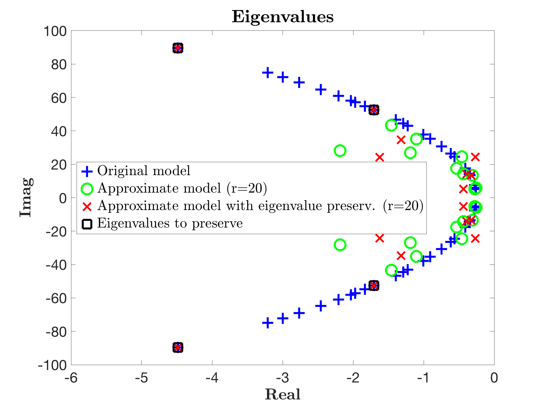
leads to the model sysr1 with state-vector of dimension 20. This leads then to the following Bode response and eigenvalues.

If one is interested in some eigenavalues of the original model, e.g. to preserve some modal meaning, the opt.eigen option can be used as:

% Reduction with eigenvalue preservation
lambda        = eig(sys); % list of eigenvalues of the original system
lambda        = lambda(imag(lambda)>0); % list of positive eigenvalues
idx           = [1 10];   % index of eigevalues to preserve (then they are closed by conjugation)
opt.eigen     = [lambda(idx); conj(lambda(idx))];
[sysr2,info2] = mor.lti(sys,r,opt);

figure(1), hold on
mor.bode(sysr2,'r--',W);
legend('Original model',['Approximate model (r=' num2str(r) ')'],['Approximate model with eigenvalue preserv. (r=' num2str(r) ')'],'Location','South')

figure(2), hold on
mor.eigen(sysr2,'rx'), hold on
plot(real(opt.eigen),imag(opt.eigen),'ks')
legend('Original model',['Approximate model (r=' num2str(r) ')'],['Approximate model with eigenvalue preserv. (r=' num2str(r) ')'],'Eigenvalues to preserve','Location','West')
xlim([-6 0]);

Leading to the following Bode response and eigenvalues, which clearly now approximate while keeping in the reduced model, the required modes. Obviously, the approximation is less accurate, but the selected modal content is preserved.