Stability estimation from frequency-domain data with MATLAB

We evaluate the stability of a linear system of dimension 2, including two delays affecting the internal variables, tau and r. The resulting system is said to be of infinite dimension because it has an infinite number of singularities. These systems are particularly complicated to analyze. Here, the considered system represents a congestion problem ni a network, and is detailled and analyzed in the article [IEEE CSM, eq. (50)].

% Test model, congestion system G(s,tau,r)
A0      = [0 0; 1 0];
A1      = [0 -2; 0 0];
A2      = [0 1.75; 0 0];
B       = [1; 0];
C       = [0 1];
tauBnd  = [0 1.4];
rBnd    = [0 1.8];
G       = @(s,tau,r) C*((s*eye(2)-A0-A1*exp(-s*tau)-A2*exp(-s*(tau+r)))\B);

From the above description of the function G, and more specifically its frequency reponse evaluation, it is possible to estimate the system stability property, thanks to the mdspack.fdstabest routine. In the considered case, we evaluate the stability for a collection of tau and r combinations, e.g. in the following manner.

% Evaluation the stability of G for frozen (tau,r)
w       = logspace(-2,1,200);
tau     = linspace(tauBnd(1),tauBnd(2),31);
r       = linspace(rBnd(1),rBnd(2),30);
for i1 = 1:numel(tau)
    for i2 = 1:numel(r)
        Gi              = @(s) G(s,tau(i1),r(i2)); 
        F               = mdspack.freqresp(Gi,w);
        [stab,Hr]       = mdspack.fdstabest(w,F);
        stabEst(i1,i2)  = stab;
    end
end
[X,Y] = meshgrid(r,tau);
figure, hold on
surf(X,Y,double(stabEst),'EdgeColor','none')
xlabel('$r$ [s]'); ylabel('$\tau$ [s]')
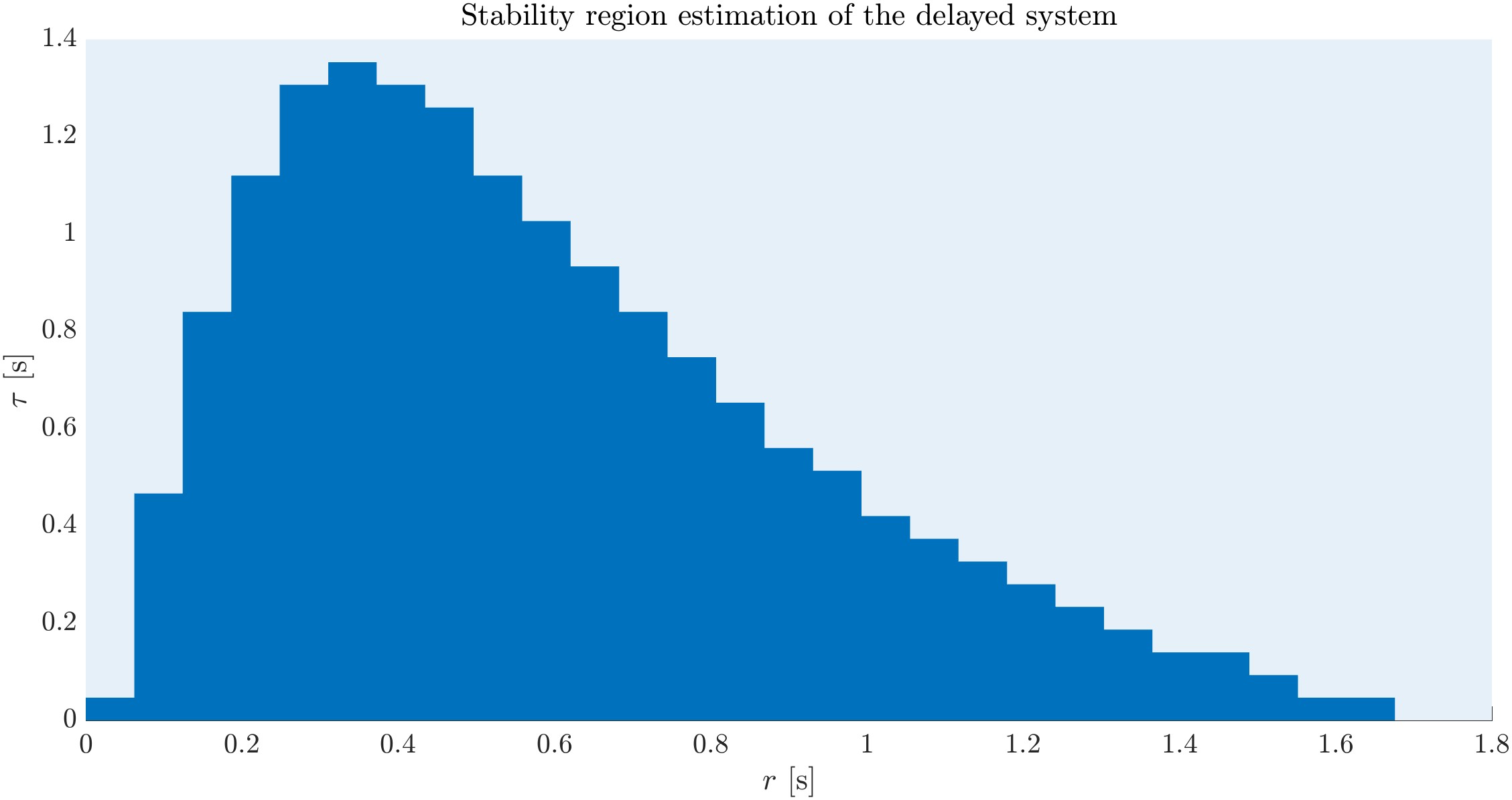
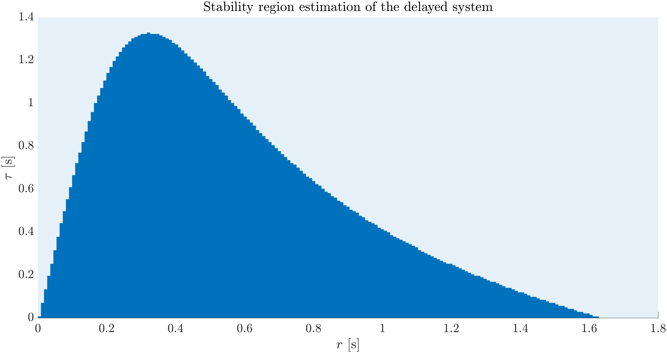
title('Stability region estimation of the delayed system')
colormap sky

The above double loop allows the construction of the stability matrix stabEst, with entries being either 1 (for stable configurations) or 0 (for unstable configurations). The figure below shows the stability region (dark blue) and the unstable one (light grey). When comparing this figure with the result described in [IEEE CSM, Figure 20], one can appreciate the similarity.

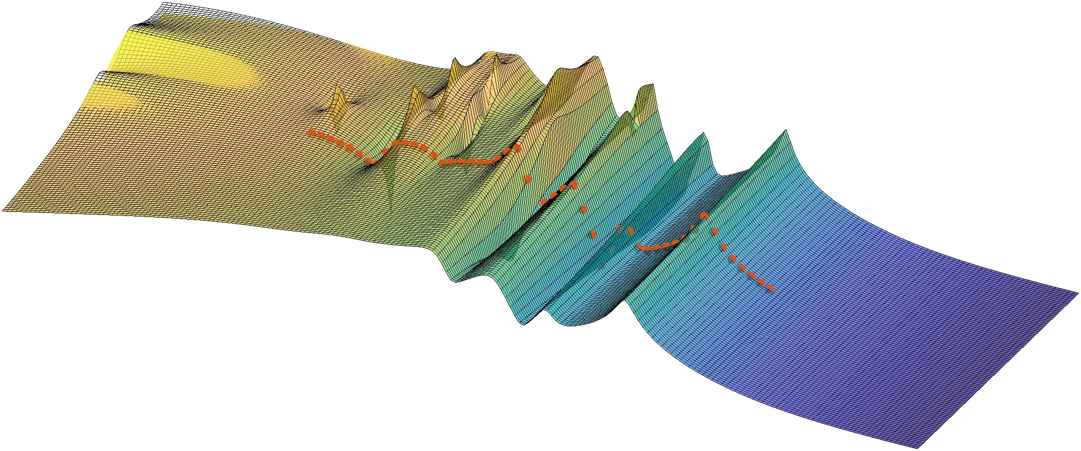
If, instead of the 31x30 gridding used above, one uses a thiner 301x300 grid, the following figure is obtained, extremely close to the theoretical result illustrated in [IEEE CSM, Figure 20].

It is also interesting comparing the stable approximating rational models, obtained mdspack.fdstabest, for two different configurations, one stable and the other unstable. In this case, let us chose the stable case (tau=1,r=0.5) and the unstable one (tau=1,r=0.6).

% Test model G(s,1,.5) and G(s,1,.6)
G1              = @(s) G(s,1,.5);
G2              = @(s) G(s,1,.6);
F1              = mdspack.freqresp(G1,w);
F2              = mdspack.freqresp(G2,w);
[stab1,Hr1]     = mdspack.fdstabest(w,F1);
[stab2,Hr2]     = mdspack.fdstabest(w,F2);

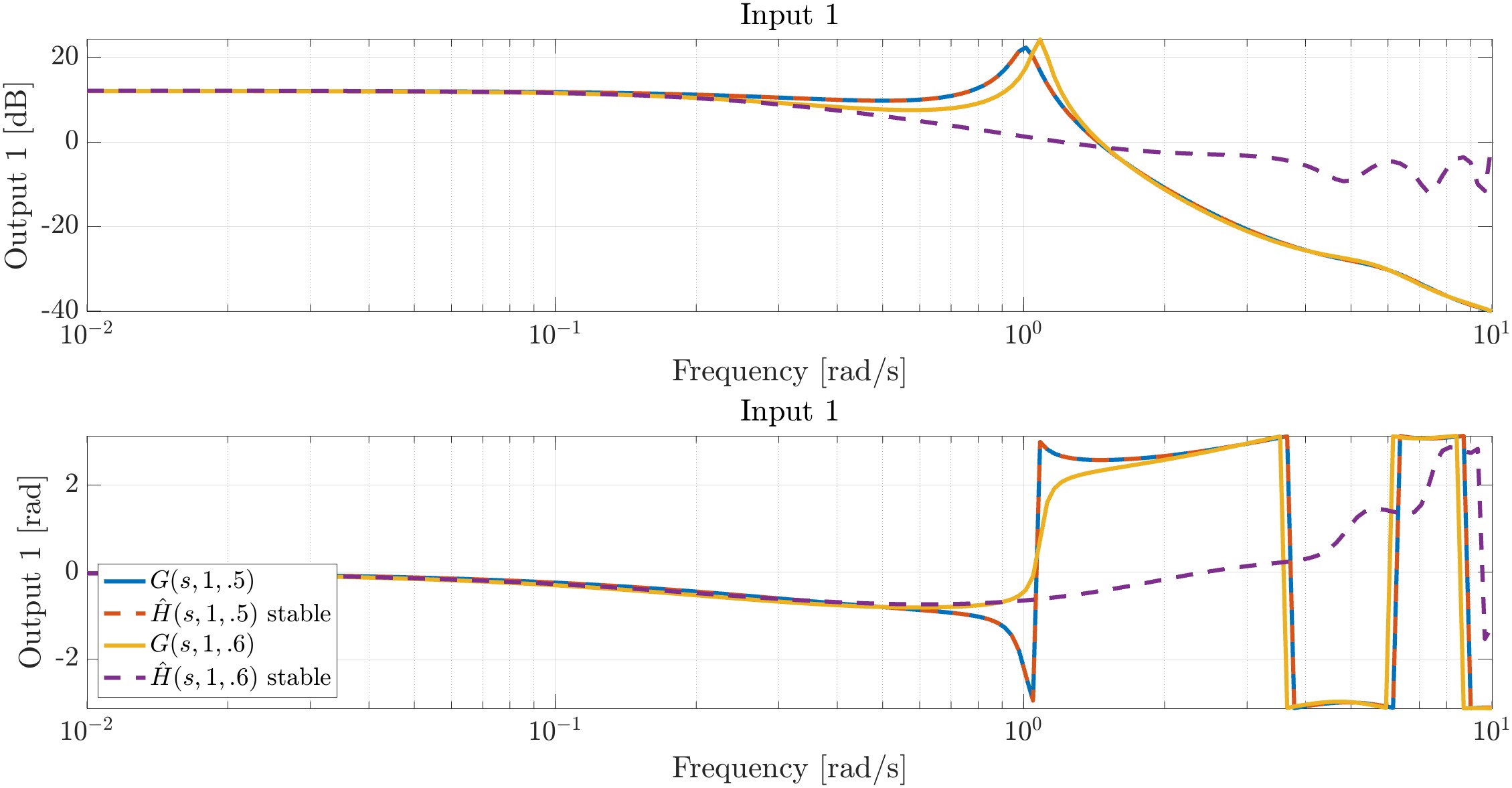
Here we notice that the frequency response of Hr1 (stable) is close to F1, being the frequency response of the stable configuration G(s,1,.5). On the other side, the frequency reponse of Hr2 (stable) is very different from F2, being the frequency response of the unstable configuration G(s,1,.6). Finally, it also interetsing to notice that the method can be applied to way more complex setup, including more delays, larger internal variables, and other complex functions, majing this solution applicable to a wide range of practical applications.

[IEEE CSM] R. Sipahi, S-I. Niculescu, C.T. Abdallah, W. Michiels, K. Gu, "Stability and stabilization of systems with time delay", IEEE Control Systems Magazine 31(1), 38-65.

Approximation/identification of a linear dynamical model, from frequency-domain data with MATLAB

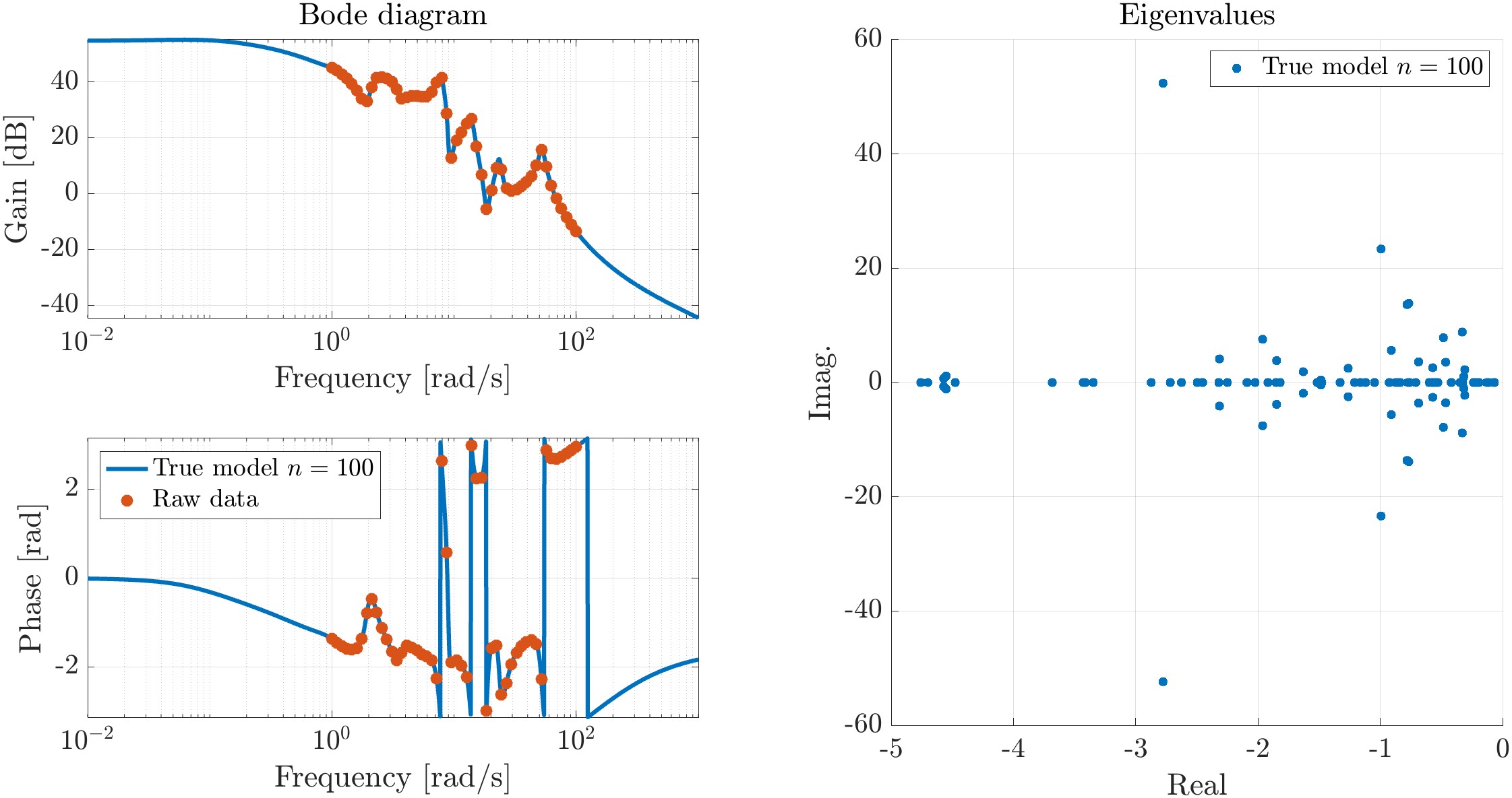
We randomly generate a single-input single-output (stable) dynamical system. This dynamical system is described by a state-space realization of dimension 100, that is, described by 100 state equations and one outpout equation. Remark: due to the use of the stabsep command, some internal variables may be eliminated.

% Create an unknown model and compute its eigenvalues
G    = stabsep(rss(200,1,1));
eigG = eig(G);

This system is considered as unknown, however, we consider that it can be evaluated. Here, it is evaluated in the frequency-domain, and more particularly along with 50 frequencies from 1 rad/s to 100 rad/s, using the mdspack.freqresp function (extension of the freqresp MATLAB function). Such an evaluation is equivalent to exciting the system with a time-domain signal (exciting this frequency interval), then applying a Fourier transform.

% Compute the associated frequency domain set
w   = logspace(0,2,50);
Gjw = mdspack.freqresp(G,w);

The figure below illustrates the frequency response (Bode diagram - gain and phase) of the original (unknow) system, as well as its evaluation (the data) we consider as known. In addition, the rigth frame shows the original system's eigenvalues (also unknown).

Thanks to the MDSPACK library and the mdspack.loewner fonction, it is possible to construct a rational approximant directly from the data. Numerically, the approximant may be result to be unstable, in this case, it is also possible to enforce the stability property thanks to mdspack.sproj.

% Data interpolation with the Loewner method
[Gr1,info1] = mdspack.loewner(w,Gjw);
% Enforce identified model stability, and eigenvalues computation
opt.space   = 'I';
Gr1         = mdspack.sproj(Gr1,opt);
eigGr1      = eig(Gr1);

The Bode diagram and eigenvalues of the identified model are then given in the below figure:

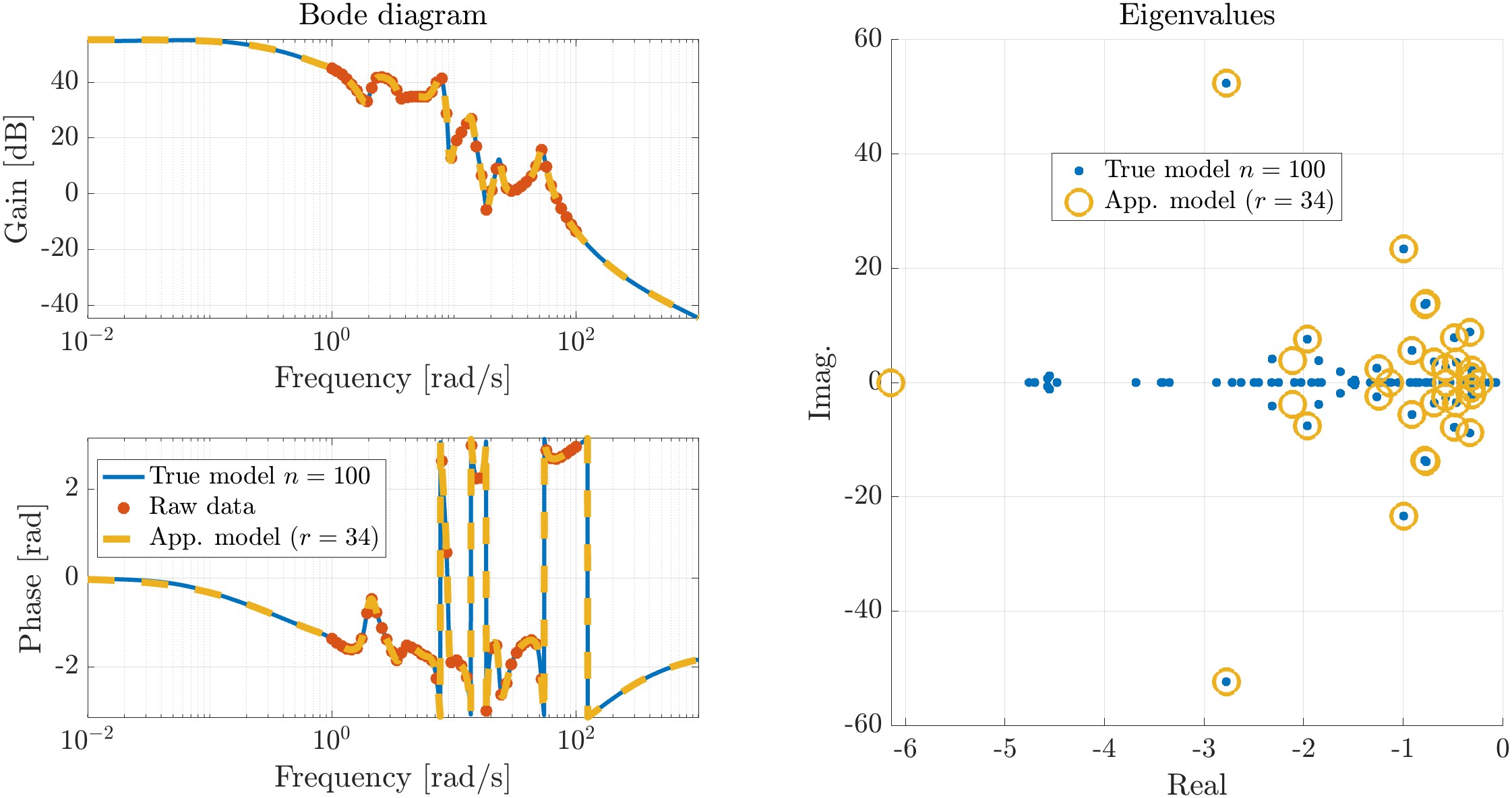
Here notice that the model's order (i.e. its complexity) is automatically chosen. In our case, the number of available data allow recovering the behaviour of the model with a machine precision. In addition, in order to simplify the analysis, it is also possible to reduce the model's complexity in the following manner (here we seek for a model with 20 states).

% Reduce the model complexity
[Gr2,info2] = mdspack.loewner(w,Gjw,struct('target',20));
Gr2         = mdspack.sproj(Gr2,struct('space','I'));
eigGr2      = eig(Gr2);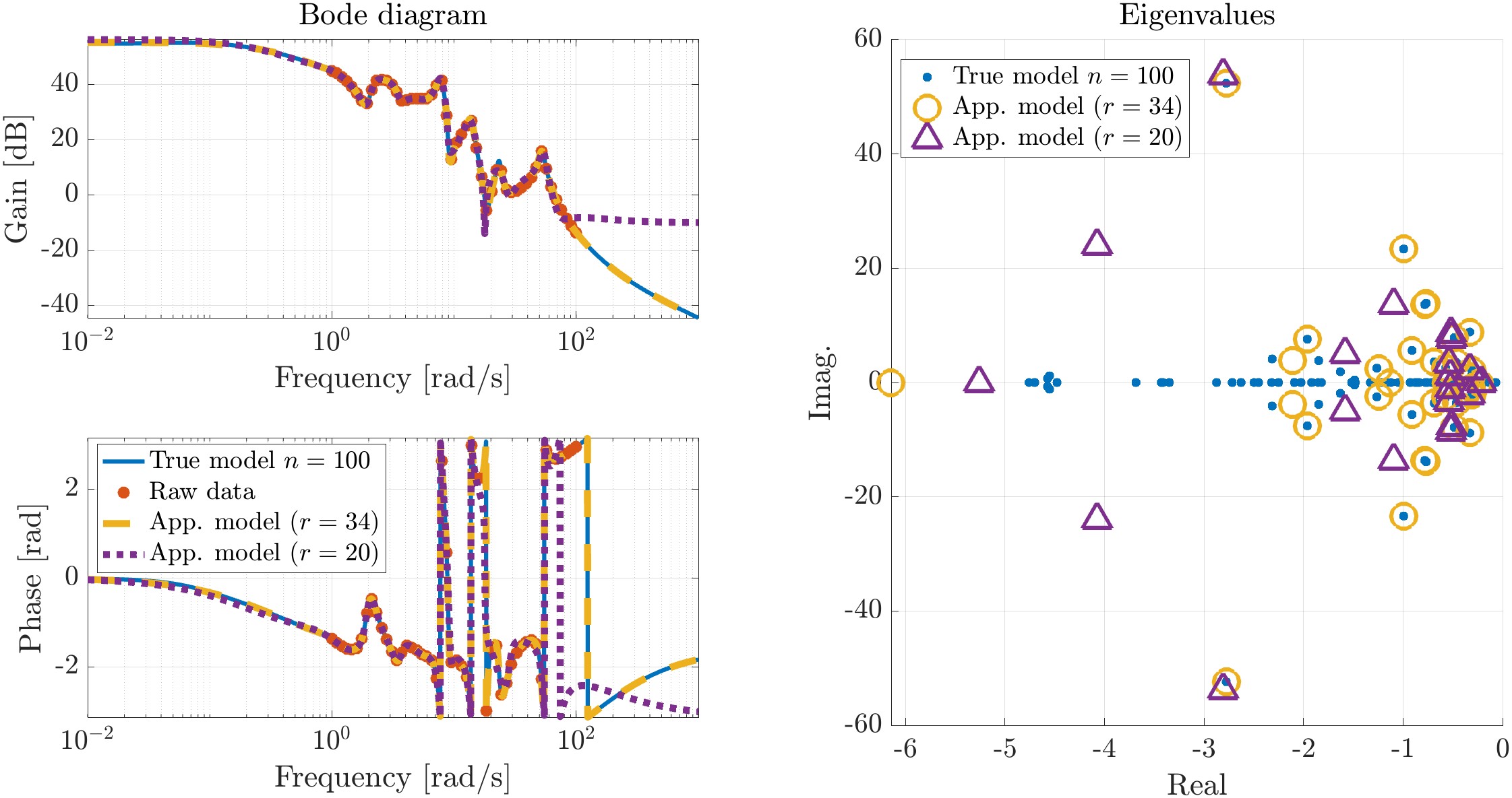

Similarly, we can also focus the approximation over a frequency domain, allowing to simplify the model by preserving the precision over the frequency range of interest. Here we seek for low frequencies. This is of particular interest when one needs to simulate a subset of the system's phenomonon only.

% Reduce over frequency band range
[Gr3,info3] = mdspack.loewner(w,Gjw,struct('w_band',[0 4]));
Gr3         = mdspack.sproj(Gr3,struct('space','I'));
eigGr3      = eig(Gr3);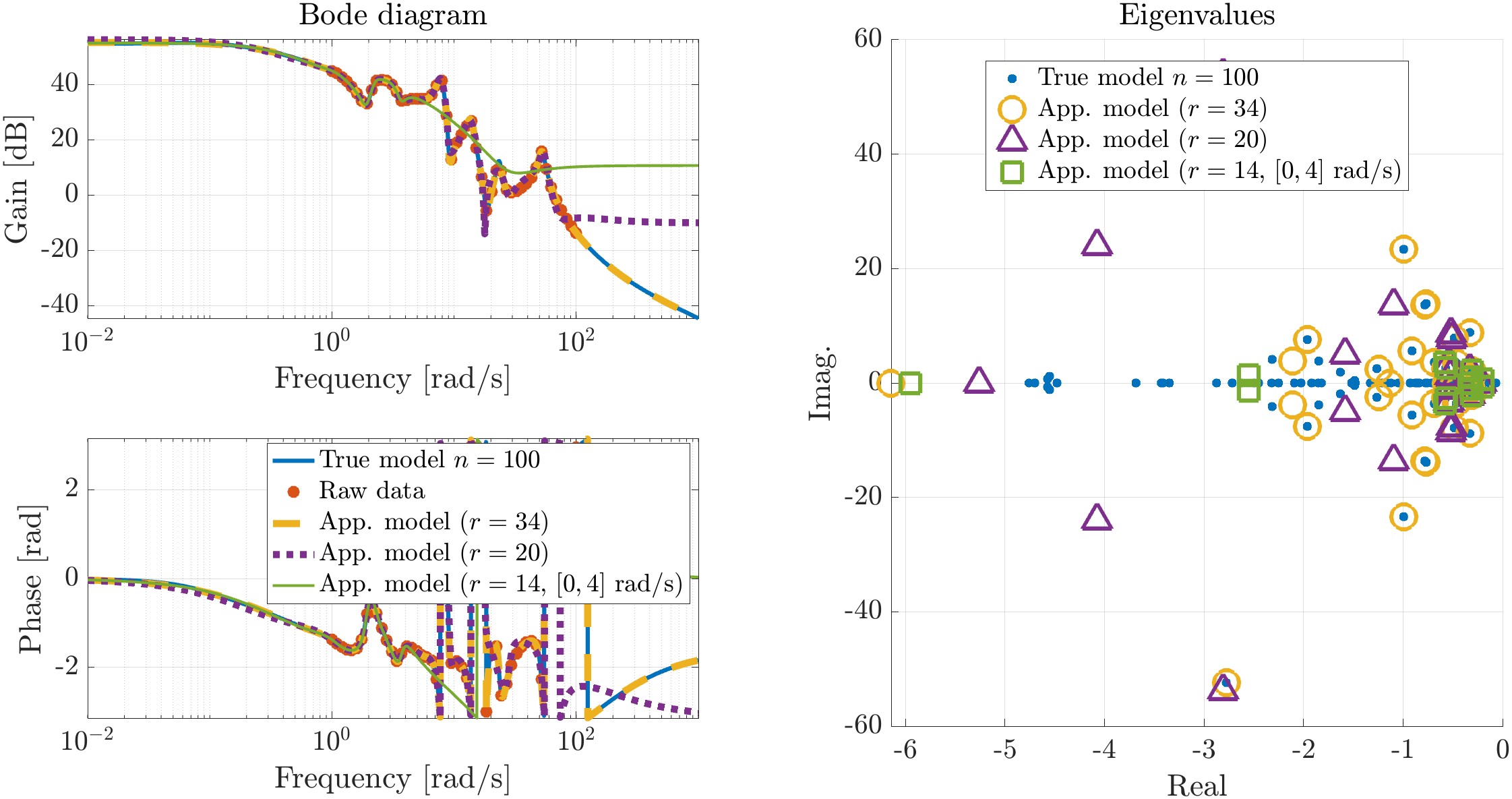

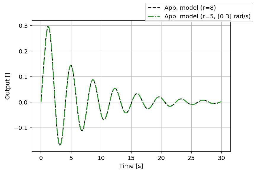
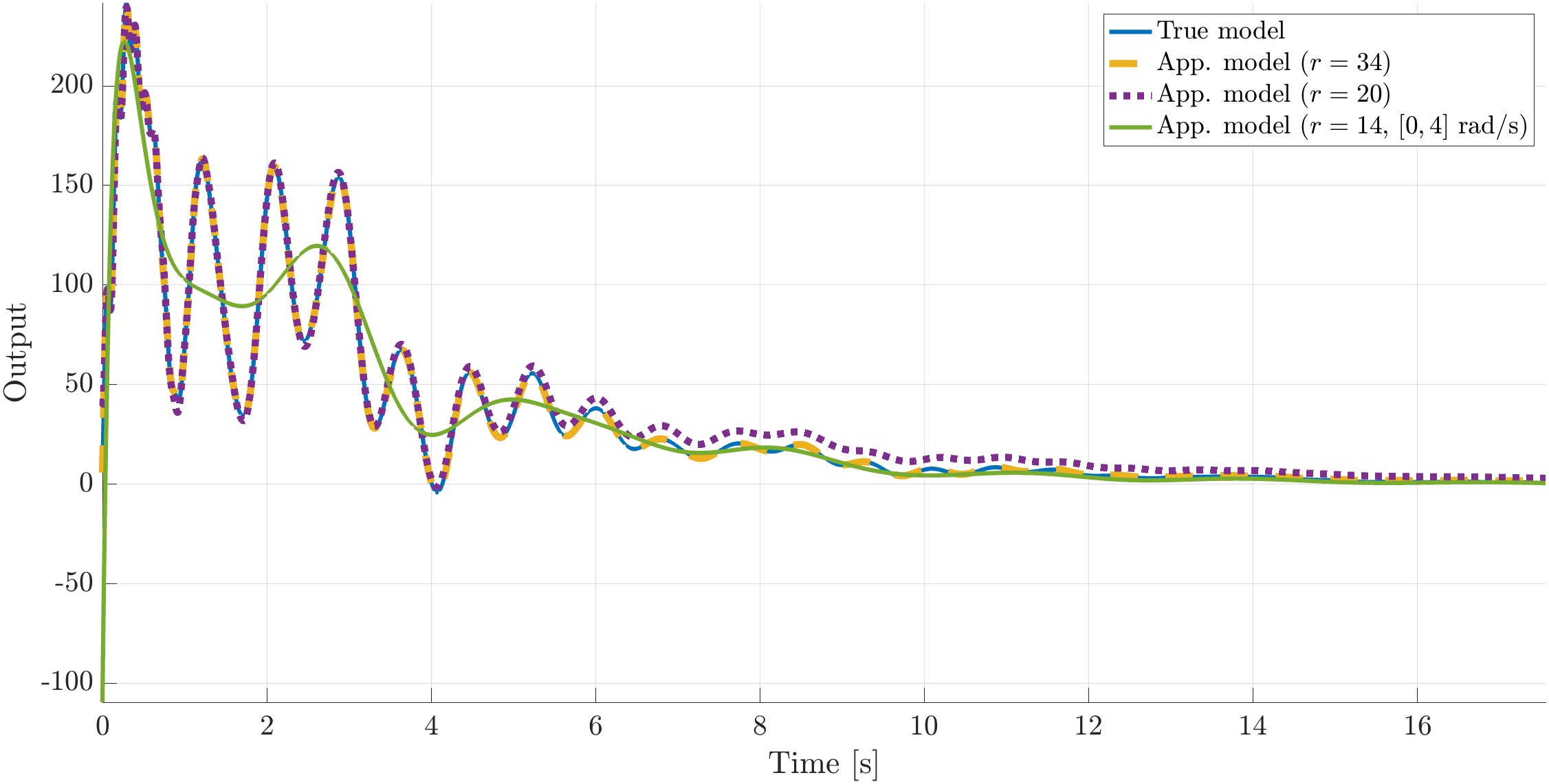
It is now possible to compare the impulse responses of the different models. It can be noticed that the first identified model very accurately captures the original one. The second one gives an approximation that preserves the trend and oscillations. The last one, which focusses on the low frequencies only, only restitues the trends and excludes the high frequency oscillations, i.e. around 1.3 Hz (or about 8 rad/s).

Approximation/identification of a linear dynamical model, from frequency-domain data with Python

Here we generate a single-input single-output (stable) dynamical system of infinite dimension. This dynamical system is described by a transfer funcion, i.e. a complex-valued funtcion linking an input to an output. Remark: this transfer function is said to be of infinite dimension because it is analytoc and its denominator has an infinite number of singularities (due to the exponential term, typically encountered in so called delay dynamical systems)

% Create an unknown model 
den = lambda s: (s**2 + s*np.exp(-4/5*s) + 1)
Hs  = lambda s: (s**1/3)/den(s)#(s**1/3)/den(s)

This system is considered as unknown, but can be evaluated. Here it is sampled along the Laplace "s" variable, along with the imaginary axis, which is equivalent in a frequency sampling. More sepcifically, 15 frequencies ranging from 0.1 rad/s to 31 rad are computed. Such an evaluation is equivalent in exciting the system with a time-domain signal (rich in frequency within this interval), then in applying the Fourier transform.

% Compute the associated frequency domain set
n       = 15
w       = list(np.logspace(-.5,1,n)) 
data    = [0 for i in range(n)]
for i in range(n):
data[i] = [[Hs(complex(0,w[i]))]]

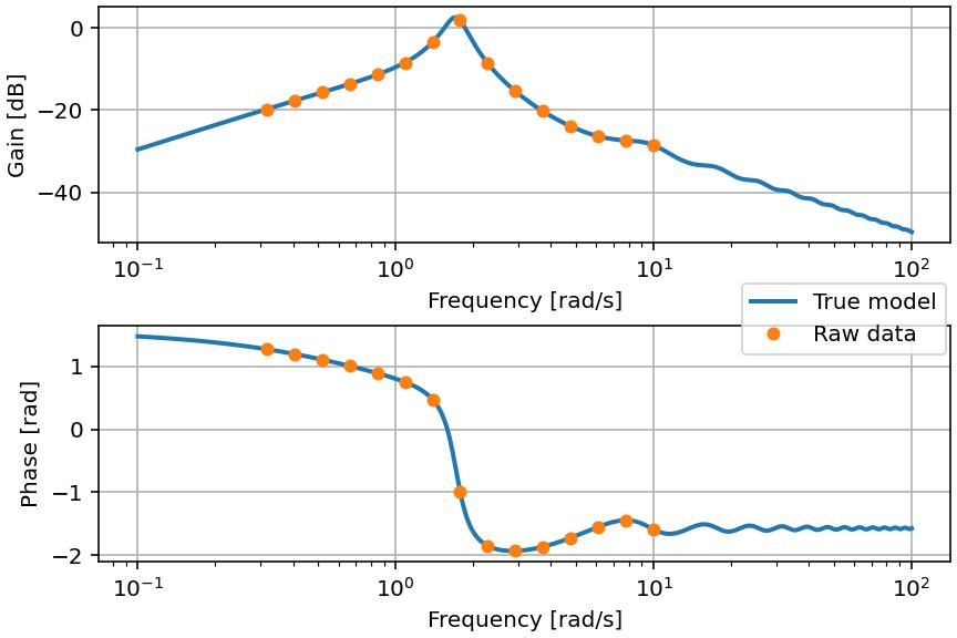
The figure below illustrates the frequency response (Bode diagram - gain and phase) of the (unknown) original system, as well as the evaluation (data) we have access. It is to be noticed that the response that we want to restitutes is irrational, and that the data we have are quite few.

Thanks to the MDSPACK library and the mdspacky.loewner function, it is possible to find a rational approximation rationnelle directly from the data. Considering that the approximant may result unstable, it is also possible to enforce stability using the available options; here ici stable=True. Then, the frequency response may be evaluated by mean of mdspacky.ssfr.

% Data interpolation with the Loewner method
[A1, B1, C1, D1, E1]    = mdspacky.loewner(w, data, stable=True)
Hjw1                    = mdspacky.ssfr(A1, B1, C1, D1, E1, W)
eigHr1                  = linalg.eigvals(A1, E1)

The Bode diagram of the original and identified models are given in the following figure:

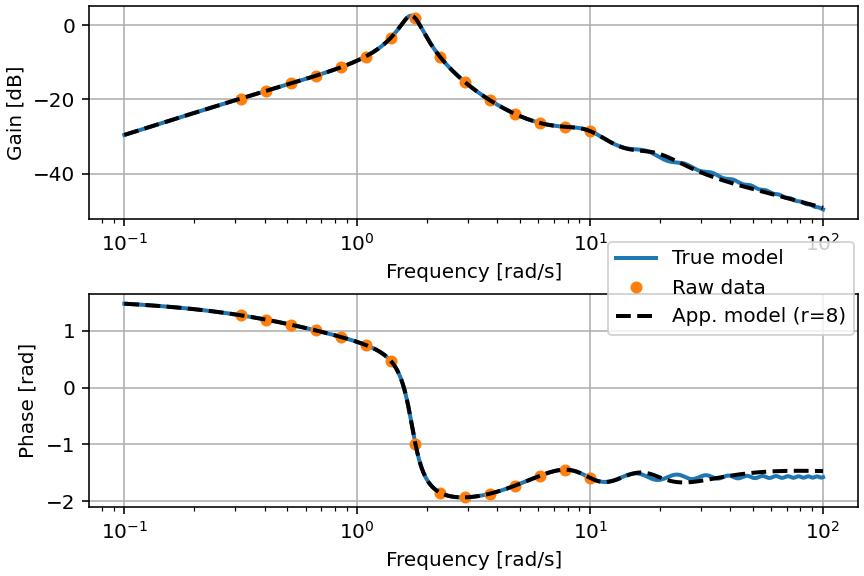
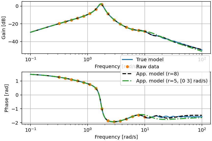
One may notice that the model order (i.e. its complexity) has been automatically chosen. In this case, the number of collected data is sufficient enought to recover the model with a great accuracy. Considering the fact that the original function is of infinite dimension, machine precision would be obtained with more samples, over a wider frequency range. In order to simplify its analysis, it is also possible to solely focus on a frequency range, allowing to simplify the identified model, while preserving a good accuracy with the domain of interest. Here, we seek a good approximation in low frequencies. Such a choice is of particular interest for simulation and feedback control of a subset of the system.

% Reduce over frequency band range
[A2, B2, C2, D2, E2]    = mdspacky.loewner(w, data, wband=[0,2], stable=True)
Hjw2                    = mdspacky.ssfr(A2, B2, C2, D2, E2, W)
eigHr2                  = linalg.eigvals(A2, E2)

Again, the order is automatically chosen, leading to a simpler model, being still accurate within the frequency interval. The Bode diagram of the original and identified models are given in the following figure:

Now, we are ready to evaluation the step responses of the rational identified models. As the original model is irrational, the same response of the original model is way more complicated to obtain.