Problem statement

Let us consider a multiple-input multiple-output (MIMO) linear time invariant model (LTI) described by the following ordinary differential equation (ODE),

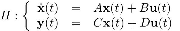
or differential algebraic equation (DAE),

where 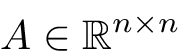, , , 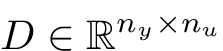and 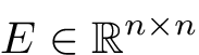(invertible), with potentially large.

Then, the objective is to determine a lower dimensional MIMO LTI model of order that well reproduces the input-output behaviour of .

Warning: unstable and limit of stability models

The model reduction algorithms are generally set for stable models. Indeed, for this case, metrics are bounded and can be exploited in the reduction procedure.

Therefore, when unstable, limit of stability or polynomial models are considered, user should consider treating them separately, i.e. to separate them from the stable model part and applying reduction on the stable part only.

Approximation interface

Let the large-scale LTI model be represented by the variablesys which can either be

• a state-space object: sys = ss(A,B,C,D) or sys = dss(A,B,C,D,E), or
• a cell containing the realisation matrices: sys = {A,B,C,D} or sys = {A,B,C,D,E} (recommanded when the model is large and sparse).

The LTI approximating model (sysr), an ODE / DAE model of order (r) can then be obtained through the unified reduction interface mor.lti as follows:

where the structure opt enables to specify the reduction options which are detailled on the mor.lti page.

Examples and how to

Perform a first model reduction

Reduce the state-space ODE / DAE dimension.

Simplify a very large-scale model

Reduce the state-space ODE / DAE dimension, when described by very large-scale (sparse) matrices.

Simplify a model over a frequency-limited band

Reduce the state-space over a frequency-limited frequency range.

Simplify a model while preserving some eigenvalues

Reduce the state-space ODE and preserves some user-defined eigenvalues/eigenvectors.